
Chapter 1: Essential Ideas
1.6 Mathematical Treatment of Measurement Results
Learning Outcomes
- Explain the dimensional analysis (factor label) approach to mathematical calculations involving quantities
- Use dimensional analysis to carry out unit conversions for a given property and computations involving two or more properties
It is often the case that a quantity of interest may not be easy (or even possible) to measure directly but instead must be calculated from other directly measured properties and appropriate mathematical relationships. For example, consider measuring the average speed of an athlete running sprints. This is typically accomplished by measuring the time required for the athlete to run from the starting line to the finish line, and the distance between these two lines, and then computing speed from the equation that relates these three properties:
[latex]\text{speed}=\dfrac{\text{distance}}{\text{time}}[/latex]
An Olympic-quality sprinter can run 100 m in approximately 10 s, corresponding to an average speed of [latex]\dfrac{\text{100 m}}{\text{10 s}}=\text{10 m/s}[/latex].
Note that this simple arithmetic involves dividing the numbers of each measured quantity to yield the number of the computed quantity (100/10 = 10) and likewise dividing the units of each measured quantity to yield the unit of the computed quantity (m/s = m/s). Now, consider using this same relation to predict the time required for a person running at this speed to travel a distance of 25 m. The same relation between the three properties is used, but in this case, the two quantities provided are a speed (10 m/s) and a distance (25 m). To yield the sought property, time, the equation must be rearranged appropriately:
[latex]\text{time}=\dfrac{\text{distance}}{\text{speed}}[/latex]
The time can then be computed as [latex]\dfrac{\text{25 m}}{\text{10 m/s}}=\text{2.5 s}[/latex].
Again, arithmetic on the numbers (25 [latex]\div[/latex] 10 = 2.5) was accompanied by the same arithmetic on the units (m/m/s = s) to yield the number and unit of the result, 2.5 s. Note that, just as for numbers, when a unit is divided by an identical unit (in this case, m/m), the result is “1”—or, as commonly phrased, the units “cancel.”
These calculations are examples of a versatile mathematical approach known as dimensional analysis (or the factor-label method). Dimensional analysis is based on this premise: the units of quantities must be subjected to the same mathematical operations as their associated numbers. This method can be applied to computations ranging from simple unit conversions to more complex, multi-step calculations involving several different quantities.
Conversion Factors and Dimensional Analysis
A ratio of two equivalent quantities expressed with different measurement units can be used as a unit conversion factor. For example, the lengths of 2.54 cm and 1 in. are equivalent (by definition), and so a unit conversion factor may be derived from the ratio,
[latex]\dfrac{\text{2.54 cm}}{\text{1 in.}}\text{(2.54 cm}=\text{1 in.) or 2.54}\dfrac{\text{cm}}{\text{in.}}[/latex]
Several other commonly used conversion factors are given in Table 1.6.1.
When a quantity (such as distance in inches) is multiplied by an appropriate unit conversion factor, the quantity is converted to an equivalent value with different units (such as distance in centimeters). For example, a basketball player’s vertical jump of 34 inches can be converted to centimeters by:
[latex]34\cancel{\text{ in.}}\times \dfrac{\text{2.54 cm}}{1\cancel{\text{in.}}}=\text{86 cm}[/latex]
Since this simple arithmetic involves quantities, the premise of dimensional analysis requires that we multiply both numbers and units. The numbers of these two quantities are multiplied to yield the number of the product quantity, 86, whereas the units are multiplied to yield [latex]\frac{\text{in.}\times \text{cm}}{\text{in.}}[/latex] . Just as for numbers, a ratio of identical units is also numerically equal to one, [latex]\frac{\text{in.}}{\text{in.}}=\text{1,}[/latex] and the unit product thus simplifies to cm. (When identical units divide to yield a factor of 1, they are said to “cancel.”) Dimensional analysis may be used to confirm the proper application of unit conversion factors as demonstrated in the following example.
Example 1.6.1: Using a Unit Conversion Factor
The mass of a competition frisbee is 125 g. Convert its mass to ounces using the unit conversion factor derived from the relationship 1 oz = 28.349 g (Table 1.6.1).
Show Solution
If we have the conversion factor, we can determine the mass in kilograms using an equation similar the one used for converting length from inches to centimeters.
[latex]x\text{ oz}=\text{125 g}\times \text{unit conversion factor}[/latex]
We write the unit conversion factor in its two forms:
[latex]\dfrac{\text{1 oz}}{\text{28.35 g}}\text{ and }\dfrac{\text{28.349 g}}{\text{1 oz}}[/latex]
The correct unit conversion factor is the ratio that cancels the units of grams and leaves ounces.
[latex]\begin{array}{ccc}x\text{ oz}\hfill & \text{=}\hfill & 125\cancel{\text{g}}\times \dfrac{\text{1 oz}}{\text{28.349}\cancel{\text{g}}}\hfill \\ \hfill & =\hfill & \left(\dfrac{125}{\text{28.349}}\right)\text{oz}\hfill \\ \hfill & =\hfill & \text{4.41 oz (three significant figures)}\hfill \end{array}[/latex]
Check Your Learning
Beyond simple unit conversions, the factor-label method can be used to solve more complex problems involving computations. Regardless of the details, the basic approach is the same—all the factors involved in the calculation must be appropriately oriented to insure that their labels (units) will appropriately cancel and/or combine to yield the desired unit in the result. This is why it is referred to as the factor-label method. As your study of chemistry continues, you will encounter many opportunities to apply this approach.
Example 1.6.2: Computing Quantities from Measurement Results and Known Mathematical Relations
What is the density of common antifreeze in units of g/mL? A 4.00 qt sample of the antifreeze weighs 9.26 lb.
Show Solution
Since [latex]\text{density}=\dfrac{\text{mass}}{\text{volume}}[/latex] , we need to divide the mass in grams by the volume in milliliters. In general: the number of units of [latex]B = \text{the number of units of } A \times \text{unit conversion factor}[/latex]. The necessary conversion factors are given in Table 1.6: 1 lb = 453.59 g; 1 L = 1.0567 qt; 1 L = 1,000 mL. We can convert mass from pounds to grams in one step:
[latex]\text{9.26}\cancel{\text{lb}}\times \dfrac{\text{453.59 g}}{1\cancel{\text{lb}}}=4.20\times {10}^{3}\text{g}[/latex]
We need to use two steps to convert volume from quarts to milliliters.
- Convert quarts to liters: [latex]\text{4.00}\cancel{\text{qt}}\times \dfrac{\text{1 L}}{\text{1.0567}\cancel{\text{qt}}}=\text{3.78 L}[/latex]
- Convert liters to milliliters: [latex]\text{3.78}\cancel{\text{L}}\times \dfrac{\text{1000 mL}}{1\cancel{\text{L}}}=3.78\times {10}^{3}\text{mL}[/latex]
Then, [latex]\text{density}=\dfrac{\text{4.20}\times {10}^{3}\text{g}}{3.78\times {10}^{3}\text{mL}}=\text{1.11 g/mL}[/latex].
Alternatively, the calculation could be set up in a way that uses three unit conversion factors sequentially as follows:
[latex]\dfrac{\text{9.26}\cancel{\text{lb}}}{\text{4.00}\cancel{\text{qt}}}\times \dfrac{\text{453.59 g}}{1\cancel{\text{lb}}}\times \dfrac{\text{1.0567}\cancel{\text{qt}}}{1\cancel{\text{L}}}\times \dfrac{1\cancel{\text{L}}}{\text{1000 mL}}=\text{1.11 g/mL}[/latex]
Check Your Learning
Example 1.6.3: Computing Quantities from Measurement Results and Known Mathematical Relations
While being driven from Philadelphia to Atlanta, a distance of about 1250 km, a 2014 Lamborghini Aventador Roadster uses 213 L gasoline.
- What (average) fuel economy, in miles per gallon, did the Roadster get during this trip?
- If gasoline costs $3.80 per gallon, what was the fuel cost for this trip?
Show Solution
Part 1
We first convert distance from kilometers to miles: [latex]\text{1250 km}\times \dfrac{\text{0.62137 mi}}{\text{1 km}}=\text{777 mi}[/latex]
Then we convert volume from liters to gallons: [latex]213\cancel{\text{L}}\times \dfrac{\text{1.0567}\cancel{\text{qt}}}{1\cancel{\text{L}}}\times \dfrac{\text{1 gal}}{4\cancel{\text{qt}}}=\text{56.3 gal}[/latex]
Then,
[latex]\text{(average) mileage}=\dfrac{\text{777 mi}}{\text{56.3 gal}}=\text{13.8 miles/gallon}=\text{13.8 mpg}[/latex]
Alternatively, the calculation could be set up in a way that uses all the conversion factors sequentially, as follows:
[latex]\dfrac{1250\cancel{\text{km}}}{213\cancel{\text{L}}}\times \dfrac{\text{0.62137 mi}}{1\cancel{\text{km}}}\times \dfrac{1\cancel{\text{L}}}{\text{1.0567}\cancel{\text{qt}}}\times \dfrac{4\cancel{\text{qt}}}{\text{1 gal}}=\text{13.8 mpg}[/latex]
Part 2
Using the previously calculated volume in gallons, we find: [latex]56.3\text{ gal}\times\dfrac{\$3.80}{1\text{ gal}}=\$214[/latex]
Check Your Learning
Conversion of Temperature Units
We use the word temperature to refer to the hotness or coldness of a substance. One way we measure a change in temperature is to use the fact that most substances expand when their temperature increases and contract when their temperature decreases. The mercury or alcohol in a common glass thermometer changes its volume as the temperature changes, and the position of the trapped liquid along a printed scale may be used as a measure of temperature.
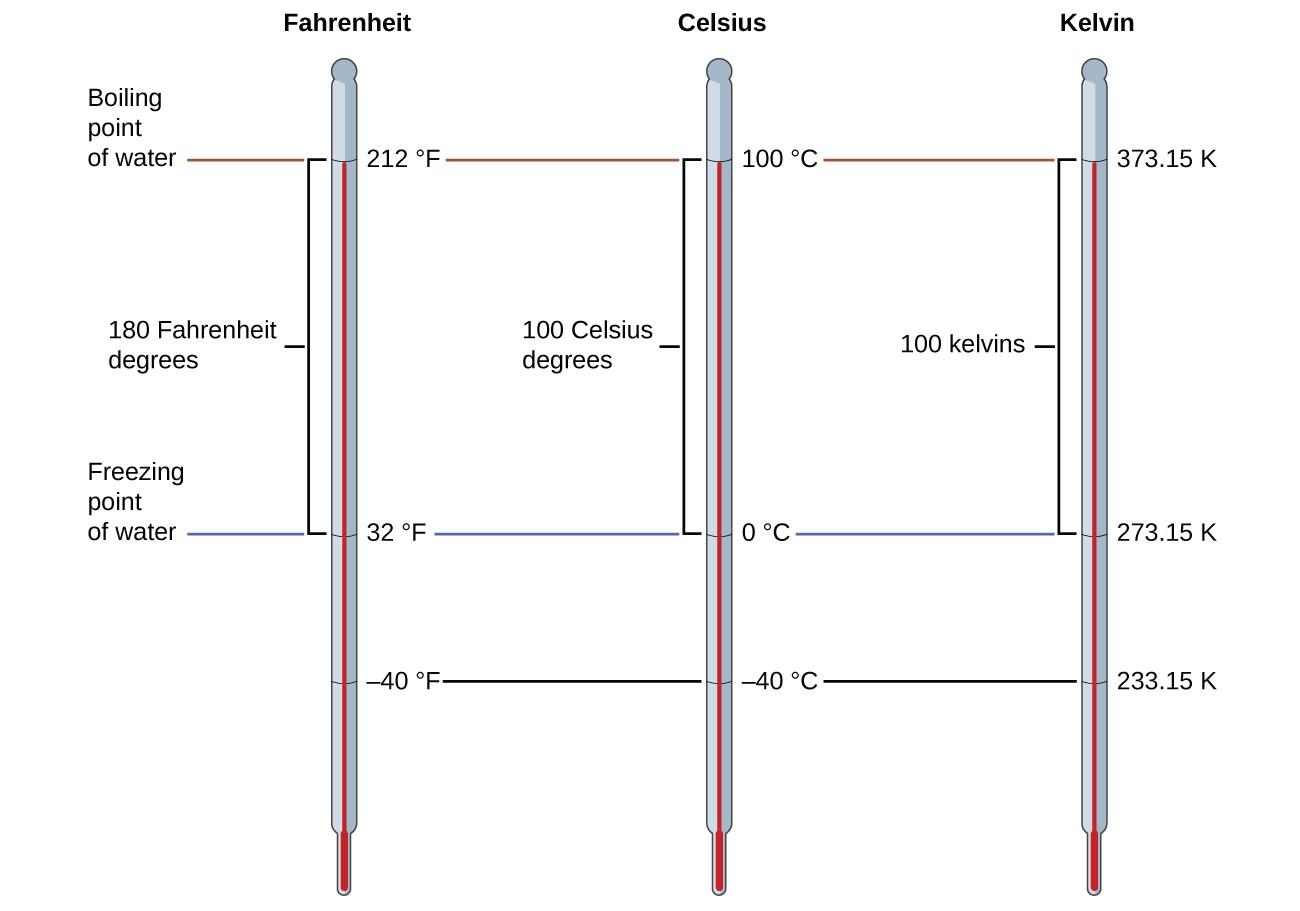
Temperature scales are defined relative to selected reference temperatures: Two of the most commonly used are the freezing and boiling temperatures of water at a specified atmospheric pressure. On the Celsius scale, 0 °C is defined as the freezing temperature of water and 100 °C as the boiling temperature of water. The space between the two temperatures is divided into 100 equal intervals, which we call degrees. On the Fahrenheit scale, the freezing point of water is defined as 32 °F and the boiling temperature as 212 °F. The space between these two points on a Fahrenheit thermometer is divided into 180 equal parts (degrees).
Defining the Celsius and Fahrenheit temperature scales as described in the previous paragraph results in a slightly more complex relationship between temperature values on these two scales than for different units of measure for other properties. Most measurement units for a given property are directly proportional to one another (y = mx). Using familiar length units as one example:
[latex]\text{length in feet}=\left(\dfrac{\text{1 ft}}{\text{12 in.}}\right)\times \text{length in inches}[/latex]
where [latex]y[/latex] = length in feet, [latex]x[/latex] = length in inches, and the proportionality constant, [latex]m[/latex], is the conversion factor. The Celsius and Fahrenheit temperature scales, however, do not share a common zero point, and so the relationship between these two scales is a linear one rather than a proportional one ([latex]y = mx + b[/latex]). Consequently, converting a temperature from one of these scales into the other requires more than simple multiplication by a conversion factor, [latex]m[/latex], it also must take into account differences in the scales’ zero points ([latex]b[/latex]).
The linear equation relating Celsius and Fahrenheit temperatures is easily derived from the two temperatures used to define each scale. Representing the Celsius temperature as [latex]x[/latex] and the Fahrenheit temperature as [latex]y[/latex], the slope, [latex]m[/latex], is computed to be:
[latex]\displaystyle{m}=\dfrac{\Delta y}{\Delta x}=\dfrac{212^{\circ}\text{ F}-32^{\circ}\text{ F}}{100^{\circ}\text{ C}-0^{\circ}\text{ C}}=\dfrac{180^{\circ}\text{ F}}{100^{\circ}\text{ C}}=\dfrac{9^{\circ}\text{ F}}{5^{\circ}\text{ C}}[/latex]
The y-intercept of the equation, [latex]b[/latex], is then calculated using either of the equivalent temperature pairs, (100 °C, 212 °F) or (0 °C, 32 °F), as:
[latex]b=y-mx=32^{\circ}\text{ F}-\dfrac{9 ^{\circ}\text{ F}}{5 ^{\circ}\text{ C}}\times{0}^{\circ}\text{ C}=32^{\circ}\text{ F}[/latex]
The equation relating the temperature scales is then:
[latex]{T}_{\text{ }^{\circ}\text{F}}=\left(\dfrac{9^{\circ}\text{ F}}{5^{\circ}\text{ C}}\times{T}_{\text{ }^{\circ}\text{C}}\right)+32 ^{\circ}\text{ C}[/latex]
An abbreviated form of this equation that omits the measurement units is:
[latex]{T}_{\text{ }^{\circ}\text{F}}=\dfrac{9}{5}\times{T}_{^{\circ}\text{ C}}+32[/latex]
We can graph that equation to visualize the relationship between Fahrenheit and Celsius:

Rearrangement of this equation yields the form most useful for converting from Fahrenheit to Celsius:
[latex]{T}_{\text{ }^{\circ}\text{C}}=\dfrac{5}{9}\left({T}_{^{\circ}\text{ F}}-32\right)[/latex]
As mentioned earlier, the SI unit of temperature is the kelvin (K). Unlike the Celsius and Fahrenheit scales, the kelvin scale is an absolute temperature scale in which 0 (zero) K corresponds to the lowest temperature that can theoretically be achieved. The early 19th-century discovery of the relationship between a gas’s volume and temperature suggested that the volume of a gas would be zero at −273.15 °C. In 1848, British physicist William Thompson, who later adopted the title of Lord Kelvin, proposed an absolute temperature scale based on this concept (further treatment of this topic is provided in the module on gases).
The freezing temperature of water on this scale is 273.15 K and its boiling temperature 373.15 K. Notice the numerical difference in these two reference temperatures is 100, the same as for the Celsius scale, and so the linear relation between these two temperature scales will exhibit a slope of [latex]1\dfrac{\text{K}}{^{\circ}\text{C}}[/latex] . Following the same approach, the equations for converting between the kelvin and Celsius temperature scales are derived to be:
[latex]{T}_{\text{K}}={T}_{^{\circ}\text{C}}+\text{273.15}[/latex]
[latex]{T}_{\text{ }^{\circ}\text{C}}={T}_{\text{K}}-\text{273.15}[/latex]
The 273.15 in these equations has been determined experimentally, so it is not exact. Figure 1.6.2 shows the relationship among the three temperature scales. Recall that we do not use the degree sign with temperatures on the kelvin scale.
Although the kelvin (absolute) temperature scale is the official SI temperature scale, Celsius is commonly used in many scientific contexts and is the scale of choice for nonscience contexts in almost all areas of the world. Very few countries (the U.S. and its territories, the Bahamas, Belize, Cayman Islands, and Palau) still use Fahrenheit for weather, medicine, and cooking.
Example 1.6.4: Conversion from Celsius
Normal body temperature has been commonly accepted as 37.0 °C (although it varies depending on time of day and method of measurement, as well as among individuals). What is this temperature on the kelvin scale and on the Fahrenheit scale?
Show Solution
[latex]\text{K}=\text{ }^{\circ}\text{C}+273.15=37.0+273.2=\text{310.2 K}[/latex]
[latex]\text{ }^{\circ}\text{F}=\dfrac{9}{5}^{\circ}\text{ C}+32.0=\left(\dfrac{9}{5}\times 37.0\right)+32.0=66.6+32.0=98.6^{\circ}\text{ F}[/latex]
Check Your Learning
Example 1.6.5: Conversion from Fahrenheit
Baking a ready-made pizza calls for an oven temperature of 450 °F. If you are in Europe, and your oven thermometer uses the Celsius scale, what is the setting? What is the kelvin temperature?
Show Solution
[latex]\text{ }^{\circ}\text{C}=\dfrac{5}{9}(^{\circ}\text{ F}-\text{32)}=\dfrac{5}{9}\left(450-32\right)=\dfrac{5}{9}\times 418=232^{\circ}\text{ C}\rightarrow\text{set oven to 230}^{\circ}\text{ C}\left(\text{two significant figures}\right)[/latex]
[latex]\text{K}=\text{ }^{\circ}\text{ C}+273.15=230+273=\text{503 K}\rightarrow 5.0\times {10}^{2}\text{K}\left(\text{two significant figures}\right)[/latex]
Check Your Learning
Key Concepts and Summary
Measurements are made using a variety of units. It is often useful or necessary to convert a measured quantity from one unit into another. These conversions are accomplished using unit conversion factors, which are derived by simple applications of a mathematical approach called the factor-label method or dimensional analysis. This strategy is also employed to calculate sought quantities using measured quantities and appropriate mathematical relations.
Key Equations
- [latex]{T}_{^{\circ}\text{C}}=\dfrac{5}{9}\times {T}_{^{\circ}\text{F}}-32[/latex]
- [latex]{T}_{^{\circ}\text{F}}=\dfrac{9}{5}\times {T}_{^{\circ}\text{C}}+32[/latex]
- [latex]{T}_{\text{K}}=\text{ }^{\circ}\text{C}+273.15[/latex]
- [latex]{T}_{^{\circ}\text{C}}=\text{K}-273.15[/latex]
Try It
- Calculate these volumes.
-
- What is the volume of 11.3 g graphite, density = 2.25 g/cm3?
- What is the volume of 39.657 g bromine, density = 2.928 g/cm3?
-
- Convert the boiling temperature of gold, 2966 °C, into degrees Fahrenheit and kelvin.
- Use scientific (exponential) notation to express the following quantities in terms of the SI base units in Table 1.6.1:
-
- 0.13 g
- 232 Gg
- 5.23 pm
-
- Complete the following conversions between SI units.
-
- 612 g = ________ mg
- 8.160 m = ________ cm
- 3779 μg = ________ g
-
Show Selected Solutions
- 5371 °F, 3239 K
-
- 1.3 × 10[latex]-[/latex]4 kg
- 2.32 × 10⁸ kg
- 5.23 × 10[latex]-[/latex]12 m
- 8.63 × 10[latex]-[/latex]5 kg
- 3.76 × 10[latex]-[/latex]1 m
- 5.4 × 10[latex]-[/latex]5 m
- 1 × 10¹² s
- 2.7 × 10[latex]-[/latex]11 s
- 1.5 × 10[latex]-[/latex]4 K
Glossary
dimensional analysis: (also, factor-label method) versatile mathematical approach that can be applied to computations ranging from simple unit conversions to more complex, multi-step calculations involving several different quantities
Fahrenheit: unit of temperature; water freezes at 32 °F and boils at 212 °F on this scale
unit conversion factor: ratio of equivalent quantities expressed with different units; used to convert from one unit to a different unit
Licenses and Attributions (Click to expand)
CC licensed content, Shared previously
- Chemistry 2e. Provided by: OpenStax. Located at: https://openstax.org/. License: CC BY: Attribution. License Terms: Access for free at
https://openstax.org/books/chemistry-2e/pages/1-introduction
All rights reserved content
- Atom Bombs and Dimensional Analysis – Sixty Symbols. Authored by: Sixty Symbols. Located at: https://youtu.be/_gaCAFcW6OY. License: Other. License Terms: Standard YouTube License
(also, factor-label method) versatile mathematical approach that can be applied to computations ranging from simple unit conversions to more complex, multi-step calculations involving several different quantities
ratio of equivalent quantities expressed with different units; used to convert from one unit to a different unit
unit of temperature; water freezes at 32 °F and boils at 212 °F on this scale
