
Chapter 3: The Quantum-Mechanical Model of the Atom
3.5 Quantum Mechanics and The Atom – Chemistry LibreTexts
https://chem.libretexts.org/Bookshelves/General_Chemistry/Map%3A_A_Molecular_Approach_(Tro)/07%3A_The_Quantum-Mechanical_Model_of_the_Atom/7.05%3A_Quantum_Mechanics_and_The_Atom
Learning Objectives
- To apply the results of quantum mechanics to chemistry.
- List and describe traits of the four quantum numbers that form the basis for completely specifying the state of an electron in an atom
The paradox described by Heisenberg’s uncertainty principle and the wavelike nature of subatomic particles such as the electron made it impossible to use the equations of classical physics to describe the motion of electrons in atoms. Scientists needed a new approach that took the wave behavior of the electron into account. In 1926, an Austrian physicist, Erwin Schrödinger (1887–1961; Nobel Prize in Physics, 1933), developed wave mechanics, a mathematical technique that describes the relationship between the motion of a particle that exhibits wavelike properties (such as an electron) and its allowed energies.
Although quantum mechanics uses sophisticated mathematics, you do not need to understand the mathematical details to follow our discussion of its general conclusions. We focus on the properties of the wavefunctions that are the solutions of Schrödinger’s equations.
Wavefunctions
A wavefunction ([latex]\psi[/latex]) is a mathematical function that relates the location of an electron at a given point in space (identified by x, y, and z coordinates) to the amplitude of its wave, which corresponds to its energy. Thus each wavefunction is associated with a particular energy E. The properties of wavefunctions derived from quantum mechanics are summarized here:
-
- A wavefunction uses three variables to describe the position of an electron. A fourth variable is usually required to fully describe the location of objects in motion. Three specify the position in space (as with the Cartesian coordinates x, y, and z.), and one specifies the time at which the object is at the specified location. For example, if you were the captain of a ship trying to intercept an enemy submarine, you would need to know its latitude, longitude, and depth, as well as the time at which it was going to be at this position (Figure 3.5.1). For electrons, we can ignore the time dependence because we will be using standing waves, which by definition do not change with time, to describe the position of an electron.
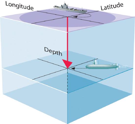
Figure 3.5.1: The Four Variables (Latitude, Longitude, Depth, and Time) required to precisely locate an object
- A wavefunction uses three variables to describe the position of an electron. A fourth variable is usually required to fully describe the location of objects in motion. Three specify the position in space (as with the Cartesian coordinates x, y, and z.), and one specifies the time at which the object is at the specified location. For example, if you were the captain of a ship trying to intercept an enemy submarine, you would need to know its latitude, longitude, and depth, as well as the time at which it was going to be at this position (Figure 3.5.1). For electrons, we can ignore the time dependence because we will be using standing waves, which by definition do not change with time, to describe the position of an electron.
The magnitude of the wavefunction at a particular point in space is proportional to the amplitude of the wave at that point. Many wavefunctions are complex functions, which is a mathematical term indicating that they contain [latex]\sqrt{-1}[/latex], represented as i. Hence the amplitude of the wave has no real physical significance. In contrast, the sign of the wavefunction (either positive or negative) corresponds to the phase of the wave, which will be important in our discussion of chemical bonding. The sign of the wavefunction should not be confused with a positive or negative electrical charge.
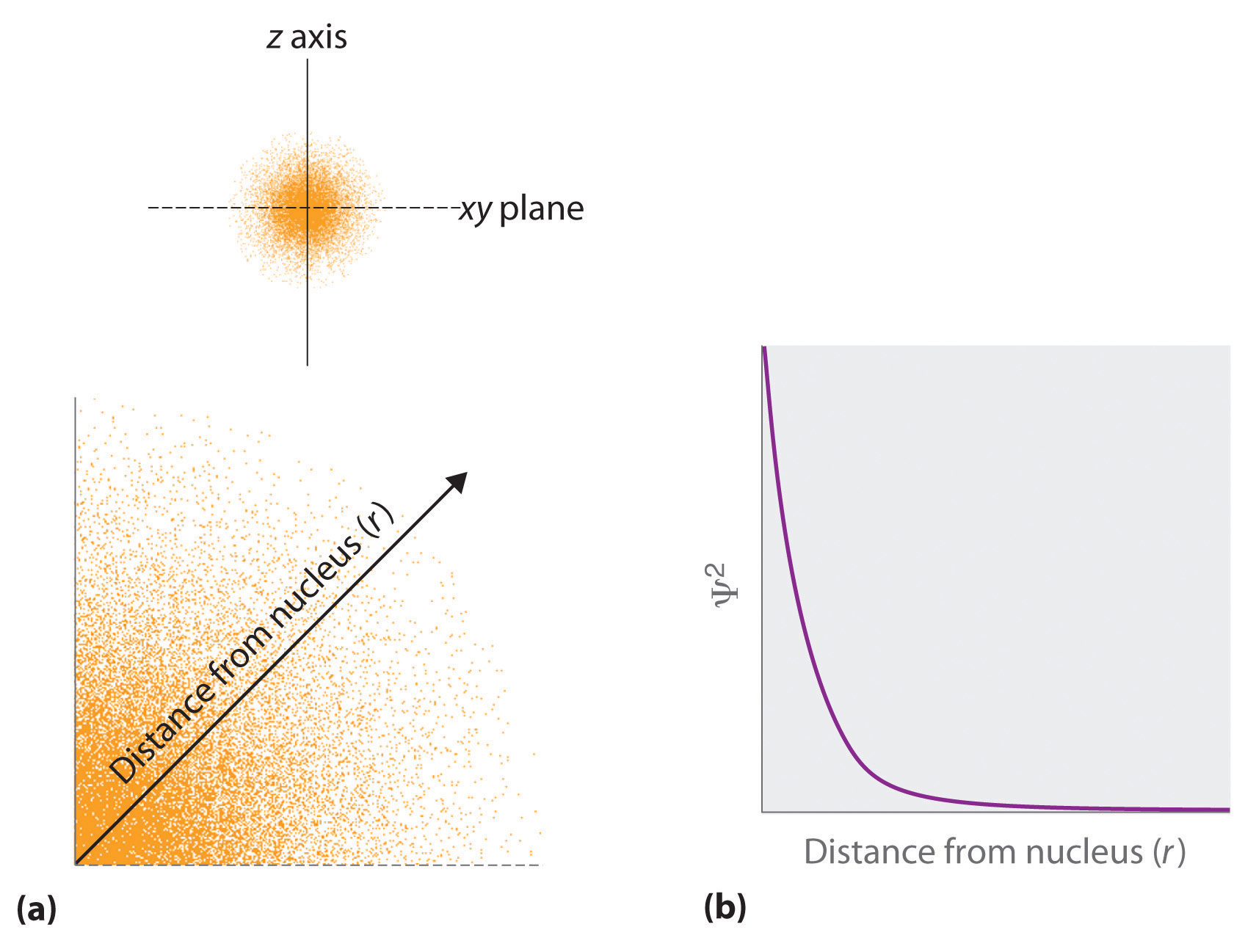
The square of the wavefunction at a given point is proportional to the probability of finding an electron at that point, which leads to a distribution of probabilities in space. The square of the wavefunction ([latex]\Psi^2[/latex]) is always a real quantity [recall that that [latex]\sqrt{-1}^2=-1[/latex]] and is proportional to the probability of finding an electron at a given point.More accurately, the probability is given by the product of the wavefunction [latex]\psi[/latex] and its complex conjugate [latex]\psi*[/latex], in which all terms that contain i are replaced by [latex]-[/latex]i. We use probabilities because, according to Heisenberg’s uncertainty principle, we cannot precisely specify the position of an electron. The probability of finding an electron at any point in space depends on several factors, including the distance from the nucleus and, in many cases, the atomic equivalent of latitude and longitude. As one way of graphically representing the probability distribution, the probability of finding an electron is indicated by the density of colored dots, as shown for the ground state of the hydrogen atom in Figure 3.5.2.
- Describing the electron distribution as a standing wave leads to sets of quantum numbers that are characteristic of each wavefunction. From the patterns of one- and two-dimensional standing waves shown previously, you might expect (correctly) that the patterns of three-dimensional standing waves would be complex. Fortunately, however, in the 18th century, a French mathematician, Adrien Legendre (1752–1783), developed a set of equations to describe the motion of tidal waves on the surface of a flooded planet. Schrödinger incorporated Legendre’s equations into his wavefunctions. The requirement that the waves must be in phase with one another to avoid cancellation and produce a standing wave results in a limited number of solutions (wavefunctions), each of which is specified by a set of numbers called quantum numbers.
- Each wavefunction is associated with a particular energy. As in Bohr’s model, the energy of an electron in an atom is quantized; it can have only certain allowed values. The major difference between Bohr’s model and Schrödinger’s approach is that Bohr had to impose the idea of quantization arbitrarily, whereas in Schrödinger’s approach, quantization is a natural consequence of describing an electron as a standing wave.
Quantum Numbers
Schrödinger’s approach uses three quantum numbers (n, l, and ml) to specify any wavefunction. The quantum numbers provide information about the spatial distribution of an electron. Although n can be any positive integer, only certain values of l and ml are allowed for a given value of n.
The Principal Quantum Number
The principal quantum number (n) tells the average relative distance of an electron from the nucleus:
n = 1, 2, 3, 4, …
As n increases for a given atom, so does the average distance of an electron from the nucleus. A negatively charged electron that is, on average, closer to the positively charged nucleus is attracted to the nucleus more strongly than an electron that is farther out in space. This means that electrons with higher values of n are easier to remove from an atom. All wavefunctions that have the same value of n are said to constitute a principal shell because those electrons have similar average distances from the nucleus. As you will see, the principal quantum number n corresponds to the n used by Bohr to describe electron orbits and by Rydberg to describe atomic energy levels.
The Angular Momentum (Azimuthal) Quantum Number
The second quantum number is often called the angular momentum (azimuthal) quantum number (l). The value of l describes the shape of the region of space occupied by the electron. The allowed values of l depend on the value of n and can range from 0 to n - 1:
l = 0, 1, 2, … , n - 1
For example, if n = 1, l can be only 0; if n = 2, l can be 0 or 1 and so forth. For a given atom, all wavefunctions that have the same values of both n and l form a subshell. The regions of space occupied by electrons in the same subshell usually have the same shape, but they are oriented differently in space.
The Magnetic Quantum Number
The third quantum number is the magnetic quantum number (ml). The value of ml describes the orientation of the region in space occupied by an electron with respect to an applied magnetic field. The allowed values of ml depend on the value of l: ml can range from -l to l in integral steps:
ml = -l, -l + 1, …, 0, …, l - 1, l
For example, if l = 0, ml can be only 0; if l = 1, ml can be -1, 0, or +1; and if l = 2, ml can be -2, -1, 0, +1, or +2.
Each wavefunction with an allowed combination of n, l, and ml values describes an atomic orbital, a particular spatial distribution for an electron. For a given set of quantum numbers, each principal shell has a fixed number of subshells, and each subshell has a fixed number of orbitals.
Example 3.5.1: n=3 and n=4 Shell Structure
How many subshells and orbitals are contained within the principal shell with n = 4?
Given: value of n
Asked for: number of subshells and orbitals in the principal shell
Strategy:
- Given n = 4, calculate the allowed values of l. From these allowed values, count the number of subshells.
- For each allowed value of l, calculate the allowed values of ml. The sum of the number of orbitals in each subshell is the number of orbitals in the principal shell.
Solution:
1 We know that l can have all integral values from 0 to n - 1. If n = 4, then l can equal 0, 1, 2, or 3. Because the shell has four values of l, it has four subshells, each of which will contain a different number of orbitals, depending on the allowed values of ml.
2 For l = 0, ml can be only 0, and thus the l = 0 subshell has only one orbital. For l = 1, ml can be 0 or ±1; thus the l = 1 subshell has three orbitals. For l = 2, ml can be 0, ±1, or ±2, so there are five orbitals in the l = 2 subshell. The last allowed value of l is l = 3, for which ml can be 0, ±1, ±2, or 3, resulting in seven orbitals in the l = 3 subshell. The total number of orbitals in the n = 4 principal shell is the sum of the number of orbitals in each subshell and is equal to n2 = 16
Check Your Learning
Rather than specifying all the values of n and l every time we refer to a subshell or an orbital, chemists use an abbreviated system with lowercase letters to denote the value of l for a particular subshell or orbital:
| l = | 0 | 1 | 2 | 3 |
|---|---|---|---|---|
| Designation | s | p | d | f |
The principal quantum number is named first, followed by the letter s, p, d, or f as appropriate. (These orbital designations are derived from historical terms for corresponding spectroscopic characteristics: sharp, principle, diffuse, and fundamental.) A 1s orbital has n = 1 and l = 0; a 2p subshell has n = 2and l = 1 (and has three 2p orbitals, corresponding to ml = -1, 0, and +1); a 3d subshell has n = 3 and l = 2 (and has five 3d orbitals, corresponding to ml = -1, -1, 0, +1, and +2); and so forth.
We can summarize the relationships between the quantum numbers and the number of subshells and orbitals as follows (Table 3.5.1):
- Each principal shell has n subshells. For n = 1, only a single subshell is possible (1s); forn = 2, there are two subshells (2s and 2p); for n = 3, there are three subshells (3s, 3p, and 3d); and so forth. Every shell has an ns subshell, any shell with n [latex]≥[/latex] 2 also has an np subshell, and any shell with n ≥ 3 also has an nd subshell. Because a 2d subshell would require both n = 2 and l = 2, which is not an allowed value of l for n = 2, a 2d subshell does not exist.
- Each subshell has 2l + 1 orbitals. This means that all ns subshells contain a single s orbital, all np subshells contain three p orbitals, all nd subshells contain five d orbitals, and all nf subshells contain seven f orbitals.
The Magnetic Quantum Number
While the three quantum numbers discussed in the previous paragraphs work well for describing electron orbitals, some experiments showed that they were not sufficient to explain all observed results. It was demonstrated in the 1920s that when hydrogen-line spectra are examined at extremely high resolution, some lines are actually not single peaks but, rather, pairs of closely spaced lines. This is the so-called fine structure of the spectrum, and it implies that there are additional small differences in energies of electrons even when they are located in the same orbital. These observations led Samuel Goudsmit and George Uhlenbeck to propose that electrons have a fourth quantum number. They called this the spin quantum number, or ms.
The other three quantum numbers, n, l, and ml, are properties of specific atomic orbitals that also define in what part of the space an electron is most likely to be located. Orbitals are a result of solving the Schrödinger equation for electrons in atoms. The electron spin is a different kind of property. It is a completely quantum phenomenon with no analogues in the classical realm. In addition, it cannot be derived from solving the Schrödinger equation and is not related to the normal spatial coordinates (such as the Cartesian x, y, and z). Electron spin describes an intrinsic electron “rotation” or “spinning.” Each electron acts as a tiny magnet or a tiny rotating object with an angular momentum, even though this rotation cannot be observed in terms of the spatial coordinates.
The magnitude of the overall electron spin can only have one value, and an electron can only “spin” in one of two quantized states. One is termed the [latex]\alpha[/latex] state, with the z component of the spin being in the positive direction of the z axis. This corresponds to the spin quantum number [latex]{m}_{s}=\frac{1}{2}[/latex]. The other is called the [latex]\beta[/latex] state, with the z component of the spin being negative and [latex]{m}_{s}=-\frac{1}{2}[/latex]. Any electron, regardless of the atomic orbital it is located in, can only have one of those two values of the spin quantum number. The energies of electrons having [latex]{m}_{s}=-\frac{1}{2}[/latex] and [latex]{m}_{s}=\frac{1}{2}[/latex] are different if an external magnetic field is applied.
Figure 3.5.3 illustrates this phenomenon. An electron acts like a tiny magnet. Its moment is directed up (in the positive direction of the z axis) for the [latex]\frac{1}{2}[/latex] spin quantum number and down (in the negative z direction) for the spin quantum number of [latex]-\frac{1}{2}[/latex]. A magnet has a lower energy if its magnetic moment is aligned with the external magnetic field (the left electron on Figure 9 and a higher energy for the magnetic moment being opposite to the applied field. This is why an electron with [latex]{m}_{s}=\frac{1}{2}[/latex] has a slightly lower energy in an external field in the positive z direction, and an electron with [latex]{m}_{s}=-\frac{1}{2}[/latex] has a slightly higher energy in the same field. This is true even for an electron occupying the same orbital in an atom. A spectral line corresponding to a transition for electrons from the same orbital but with different spin quantum numbers has two possible values of energy; thus, the line in the spectrum will show a fine structure splitting.
Example 3.5.2: Working with Shells and Subshells
Indicate the number of subshells, the number of orbitals in each subshell, and the values of l and ml for the orbitals in the n = 4 shell of an atom.
Show Solution
For n = 4, l can have values of 0, 1, 2, and 3. Thus, s, p , d, and [latex]f[/latex] subshells are found in the n = 4 shell of an atom. For l = 0 (the s subshell), ml can only be 0. Thus, there is only one 4s orbital. For l = 1 (p-type orbitals), m can have values of -1, 0, +1, so we find three [latex]4p[/latex] orbitals. For l = 2 (d-type orbitals), ml can have values of -2, -1, 0, +1, +2, so we have five 4d orbitals. When l = 3 (f-type orbitals), ml can have values of -3, -2, -2, 0, +1, +2, +3, and we can have seven 4f orbitals. Thus, we find a total of 16 orbitals in the n = 4 shell of an atom.
Check Your Learning
Example 3.5.3: Maximum Number of Electrons
Calculate the maximum number of electrons that can occupy a shell with the following n values:
- n = 2
- n = 5
- n as a variable.
Note you are only looking at the orbitals with the specified n value, not those at lower energies.
Show Solution
- When n = 2, there are four orbitals (a single 2s orbital, and three orbitals labeled 2p). These four orbitals can contain eight electrons.
- When n = 5, there are five subshells of orbitals that we need to sum:
[latex]\begin{array}{ll}&1\text{ orbitals labeled }5s\\ &3\text{ orbitals labeled }5p\\ &5\text{ orbitals labeled }5d\\ &7\text{ orbitals labeled }5f\\ \text{+}&\underline{9\text{ orbitals labeled }5g}\\ &25\text{ orbitals total }\end{array}[/latex]
Again, each orbital holds two electrons, so 50 electrons can fit in this shell.
- The number of orbitals in any shell n will equal n2. There can be up to two electrons in each orbital, so the maximum number of electrons will be 2 × n2
Check Your Learning
Example 3.5.4: Working with Quantum Numbers
Complete the following table for atomic orbitals:
| Orbital | n | l | ml degeneracy | Radial nodes (no.) |
|---|---|---|---|---|
| 4f | ||||
| 4 | 1 | |||
| 7 | 7 | 3 | ||
| 5d |
Show Solution
The table can be completed using the following rules:
- The orbital designation is n, where l = 0, 1, 2, 3, 4, 5, … is mapped to the letter sequence s, p, d, f, g, h, …,
- The ml degeneracy is the number of orbitals within an l subshell, and so is 2l + 1 (there is one s orbital, three p orbitals, five d orbitals, seven f orbitals, and so forth).
- The number of radial nodes is equal to n - l - 1.
| Orbital | n | l | ml degeneracy | Radial nodes (no.) |
|---|---|---|---|---|
| [latex]4f[/latex] | 4 | 3 | 7 | 0 |
| [latex]4p[/latex] | 4 | 1 | 3 | 3 |
| [latex]7f[/latex] | 7 | 3 | 3 | 3 |
| [latex]5d[/latex]5 | 5 | 3 | 5 | 2 |
Check Your Learning
Key Concepts and Summary
There is a relationship between the motions of electrons in atoms and molecules and their energies that is described by quantum mechanics. Because of wave–particle duality, scientists must deal with the probability of an electron being at a particular point in space. To do so required the development of quantum mechanics, which uses wavefunctions ([latex]\psi[/latex]) to describe the mathematical relationship between the motion of electrons in atoms and molecules and their energies. Wavefunctions have five important properties:
- the wavefunction uses three variables (Cartesian axes x, y, and z) to describe the position of an electron;
- the magnitude of the wavefunction is proportional to the intensity of the wave;
- the probability of finding an electron at a given point is proportional to the square of the wavefunction at that point, leading to a distribution of probabilities in space that is often portrayed as an electron density plot;
- describing electron distributions as standing waves leads naturally to the existence of sets of quantum numbers characteristic of each wavefunction; and
- each spatial distribution of the electron described by a wavefunction with a given set of quantum numbers has a particular energy.
The properties and meaning of the quantum numbers of electrons in atoms are briefly summarized in Table 3.5.2.
Quantum numbers provide important information about the energy and spatial distribution of an electron. The principal quantum number n can be any positive integer; as n increases for an atom, the average distance of the electron from the nucleus also increases. All wavefunctions with the same value of n constitute a principal shell in which the electrons have similar average distances from the nucleus. The azimuthal quantum number l can have integral values between 0 and n - 1; it describes the shape of the electron distribution. wavefunctions that have the same values of both n and l constitute a subshell, corresponding to electron distributions that usually differ in orientation rather than in shape or average distance from the nucleus. The magnetic quantum number ml can have 2l + 1 integral values, ranging from -l to +l, and describes the orientation of the electron distribution. Each wavefunction with a given set of values of n, l, and ml describes a particular spatial distribution of an electron in an atom, an atomic orbital.
Glossary
Wave mechanics: a mathematical technique that describes the relationship between the motion of a particle that exhibits wavelike properties (such as an electron) and its allowed energies
Quantum numbers: characteristic of each wavefunction
Principal quantum number (n): the average relative distance of an electron from the nucleus
Angular momentum (azimuthal) quantum number (l): The value of l describes the shape of the region of space occupied by the electron
Magnetic quantum number (ml): The value of ml describes the orientation of the region in space occupied by an electron with respect to an applied magnetic field
Atomic orbital, a particular spatial distribution for an electron.
Spin quantum number (ms): direction of the intrinsic quantum “spinning” of the electron
Licenses and Attributions (Click to expand)
CC licensed content, Shared previously
- N/A. Provided by: N/A. Located at: N/A. License: CC BY: Attribution. License Terms: N/A
