
Chapter 12: Solutions and Colloids
12.5 Colligative Properties
Learning Outcomes
- Explain the effect of adding a solute to a solvent on the physical properties of a solution (vapor pressure, boiling point, melting point, osmotic pressure)
- Qualitatively predict and calculate changes in vapor pressure of multi-component solutions
- Qualitatively predict and calculate changes in boiling point, freezing point, and osmotic pressure when two substances are mixed
The properties of a solution are different from those of either the pure solute(s) or solvent. Many solution properties are dependent upon the chemical identity of the solute. Compared to pure water, a solution of hydrogen chloride is more acidic, a solution of ammonia is more basic, a solution of sodium chloride is more dense, and a solution of sucrose is more viscous. There are a few solution properties, however, that depends only upon the total concentration of solute species, regardless of their identities. These colligative properties include vapor pressure lowering, boiling point elevation, freezing point depression, and osmotic pressure. This small set of properties is of central importance to many natural phenomena and technological applications, as will be described in this section.
Vapor Pressure Lowering
As described in the chapter on liquids and solids, the equilibrium vapor pressure of a liquid is the pressure exerted by its gaseous phase when vaporization and condensation are occurring at equal rates:
[latex]\text{liquid}\rightleftharpoons\text{gas}[/latex]
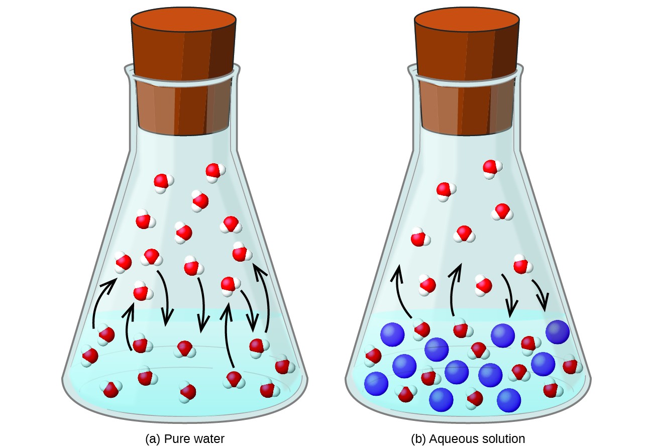
Dissolving a nonvolatile substance in a volatile liquid results in a lowering of the liquid’s vapor pressure. This phenomenon can be rationalized by considering the effect of added solute molecules on the liquid’s vaporization and condensation processes. To vaporize, solvent molecules must be present at the surface of the solution. The presence of solute decreases the surface area available to solvent molecules and thereby reduces the rate of solvent vaporization. Since the rate of condensation is unaffected by the presence of solute, the net result is that the vaporization-condensation equilibrium is achieved with fewer solvent molecules in the vapor phase (i.e., at a lower vapor pressure) (Figure 12.5.1). While this kinetic interpretation is useful, it does not account for several important aspects of the colligative nature of vapor pressure lowering. A more rigorous explanation involves the property of entropy, a topic of discussion in a later text chapter on thermodynamics. For purposes of understanding the lowering of a liquid’s vapor pressure, it is adequate to note that the greater entropy of a solution in comparison to its separate solvent and solute serves to effectively stabilize the solvent molecules and hinder their vaporization. A lower vapor pressure results, and a correspondingly higher boiling point as described in the next section of this section.
The relationship between the vapor pressures of solution components and the concentrations of those components is described by Raoult’s law: The partial pressure exerted by any component of an ideal solution is equal to the vapor pressure of the pure component multiplied by its mole fraction in the solution.
[latex]{P}_{\text{A}}={X}_{\text{A}}{P}_{\text{A}}^{ \star }[/latex]
where PA is the partial pressure exerted by component A in the solution, [latex]{P}_{\text{A}}^{\star }[/latex] is the vapor pressure of pure A, and XA is the mole fraction of A in the solution. (Mole fraction is a concentration unit introduced in the chapter on gases.)
Recalling that the total pressure of a gaseous mixture is equal to the sum of partial pressures for all its components (Dalton’s Law of partial pressures), the total vapor pressure exerted by a solution containing i components is
[latex]{P}_{\text{solution}}=\sum _{i}{P}_{i}=\sum _{i}{X}_{i}{P}_{i}^{\star}[/latex]
A nonvolatile substance is one whose vapor pressure is negligible ([latex]P^{\star}[/latex] ≈ 0), and so the vapor pressure above a solution containing only nonvolatile solutes is due only to the solvent:
[latex]{P}_{\text{solution}}={X}_{\text{solvent}}{P}_{\text{solvent}}^{\star }[/latex]
Example 12.5.1: Calculation of a Vapor Pressure
Compute the vapor pressure of an ideal solution containing 92.1 g of glycerin, [latex]\ce{C3H5(OH)3}[/latex], and 184.4 g of ethanol, [latex]\ce{C2H5OH}[/latex], at 40 °C. The vapor pressure of pure ethanol is 0.178 atm at 40 °C. Glycerin is essentially nonvolatile at this temperature.
Show Solution
Since the solvent is the only volatile component of this solution, its vapor pressure may be computed per Raoult’s law as:
[latex]{P}_{\text{solution}}={X}_{\text{solvent}}{P}_{\text{solvent}}^{ \star}[/latex]
First, calculate the molar amounts of each solution component using the provided mass data.
[latex]\begin{array}{l}\\ 92.1\cancel{\text{g}{\ce{C}}_{3}{\ce{H}}_{5}{\left(\ce{OH}\right)}_{3}}\times \dfrac{1\text{mol}{\ce{C}}_{3}{\ce{H}}_{5}{\left(\ce{OH}\right)}_{3}}{92.094\cancel{\text{g}{\ce{C}}_{3}{\ce{H}}_{5}{\left(\text{OH}\right)}_{3}}}=1.00\text{mol}{\ce{C}}_{3}{\ce{H}}_{5}{\left(\ce{OH}\right)}_{3}\\ 184.4\cancel{\text{g}{\ce{C}}_{2}{\ce{H}}_{5}\ce{OH}}\times \dfrac{1\text{mol}{\ce{C}}_{2}{\ce{H}}_{5}\ce{OH}}{46.069\cancel{\text{g}{\ce{C}}_{2}{\ce{H}}_{5}\ce{OH}}}=4.000\text{mol}{\ce{C}}_{2}{\ce{H}}_{5}\ce{OH}\end{array}[/latex]
Next, calculate the mole fraction of the solvent (ethanol) and use Raoult’s law to compute the solution’s vapor pressure.
[latex]\begin{array}{l}\\ {X}_{{\ce{C}}_{2}{\ce{H}}_{5}\ce{OH}}=\dfrac{4.000\text{mol}}{\left(1.00\text{mol}+4.000\text{mol}\right)}=0.800\\ {P}_{\text{solv}}={X}_{\text{solv}}{P}_{\text{solv}}^{ \star}=0.800\times 0.178\text{atm}=0.142\text{atm}\end{array}[/latex]
Check Your Learning
Boiling Point Elevation
As described in the chapter on liquids and solids, the boiling point of a liquid is the temperature at which its vapor pressure is equal to ambient atmospheric pressure. Since the vapor pressure of a solution is lowered due to the presence of nonvolatile solutes, it stands to reason that the solution’s boiling point will subsequently be increased. Compared to pure solvent, a solution, therefore, will require a higher temperature to achieve any given vapor pressure, including one equivalent to that of the surrounding atmosphere. The increase in boiling point observed when nonvolatile solute is dissolved in a solvent, [latex]\Delta[/latex]Tb, is called boiling point elevation and is directly proportional to the molal concentration of solute species:
[latex]\Delta{T}_{\text{b}}={K}_{\text{b}}m[/latex]
where Kb is the boiling point elevation constant, or the ebullioscopic constant and m is the molal concentration (molality) of all solute species.
Boiling point elevation constants are characteristic properties that depend on the identity of the solvent. Values of Kb for several solvents are listed in Table 12.5.1.
The extent to which the vapor pressure of a solvent is lowered and the boiling point is elevated depends on the total number of solute particles present in a given amount of solvent, not on the mass or size or chemical identities of the particles. A 1 m aqueous solution of sucrose (342 g/mol) and a 1 m aqueous solution of ethylene glycol (62 g/mol) will exhibit the same boiling point because each solution has one mole of solute particles (molecules) per kilogram of solvent.
Example 12.5.2: Calculating the Boiling Point of a Solution
What is the boiling point of a 0.33 m solution of a nonvolatile solute in benzene?
Show Solution
Use the equation relating boiling point elevation to solute molality to solve this problem in two steps.

- Calculate the change in boiling point: [latex]\Delta{T}_{\text{b}}={K}_{\text{b}}m=2.53^{\circ}\text{C }{m}^{-1}\times 0.33m=0.83^{\circ}\text{C}[/latex]
- Add the boiling point elevation to the pure solvent’s boiling point: [latex]\text{Boiling temperature}=80.1^{\circ}\text{C}+0.83^{\circ}\text{C}=80.9^{\circ}\text{C}[/latex]
Check Your Learning
Example 12.5.3: The Boiling Point of an Iodine Solution
Find the boiling point of a solution of 92.1 g of iodine, I2, in 800.0 g of chloroform, [latex]\ce{CHCl3}[/latex], assuming that the iodine is nonvolatile and that the solution is ideal.
Show Solution
We can solve this problem using four steps.

- Convert from grams to moles of I2using the molar mass of [latex]\ce{I2}[/latex] in the unit conversion factor: 0.363 mol
- Determine the molality of the solution from the number of moles of solute and the mass of solvent, in kilograms: 0.454 m
- Use the direct proportionality between the change in boiling point and molal concentration to determine how much the boiling point changes: 1.65 °C
- Determine the new boiling point from the boiling point of the pure solvent and the change: 62.91 °C. Check each result as a self-assessment.
Check Your Learning
Freezing Point Depression

Solutions freeze at lower temperatures than pure liquids. This phenomenon is exploited in “de-icing” schemes that use salt (Figure 12.5.2), calcium chloride, or urea to melt ice on roads and sidewalks, and in the use of ethylene glycol as an “antifreeze” in automobile radiators. Seawater freezes at a lower temperature than fresh water, and so the Arctic and Antarctic oceans remain unfrozen even at temperatures below 0 °C (as do the body fluids of fish and other cold-blooded sea animals that live in these oceans).
The decrease in freezing point of a dilute solution compared to that of the pure solvent, [latex]\Delta[/latex]Tf, is called the freezing point depression and is directly proportional to the molal concentration of the solute
[latex]\Delta{T}_{\text{f}}={K}_{\text{f}}m[/latex]
where m is the molal concentration of the solute in the solvent and Kf is called the freezing point depression constant (or cryoscopic constant). Just as for boiling point elevation constants, these are characteristic properties whose values depend on the chemical identity of the solvent. Values of Kf for several solvents are listed in Table 12.5.1.
Example 12.5.3: Calculation of the Freezing Point of a Solution
What is the freezing point of the 0.33 m solution of a nonvolatile nonelectrolyte solute in benzene described in Example 12.5.2?
Show Solution
Use the equation relating freezing point depression to solute molality to solve this problem in two steps.

- Calculate the change in freezing point: [latex]\Delta{T}_{\text{f}}={K}_{\text{f}}m=5.12^{\circ}\text{C}{m}^{-1}\times 0.33m=1.7^{\circ}\text{C}[/latex]
- Subtract the freezing point change observed from the pure solvent’s freezing point: [latex]\text{Freezing Temperature}=5.5^{\circ}\text{C}-1.7^{\circ}\text{C}=3.8^{\circ}\text{C}[/latex]
Check Your Learning
Phase Diagram for a Solution
The colligative effects on vapor pressure, boiling point, and freezing point described in the previous section are conveniently summarized by comparing the phase diagrams for a pure liquid and a solution derived from that liquid. Phase diagrams for water and an aqueous solution are shown in Figure 12.5.3.
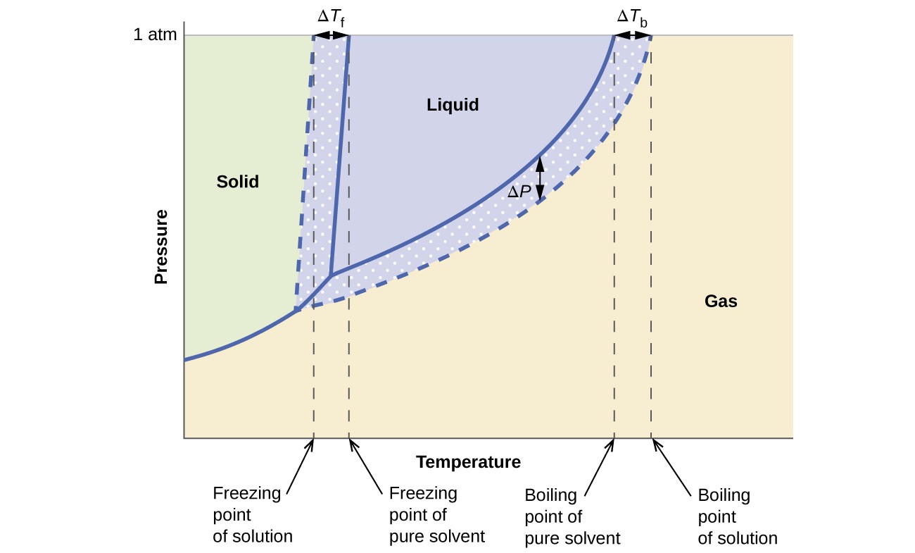
The liquid-vapor curve for the solution is located beneath the corresponding curve for the solvent, depicting the vapor pressure lowering, [latex]\Delta[/latex]P, that results from the dissolution of nonvolatile solute. Consequently, at any given pressure, the solution’s boiling point is observed at a higher temperature than that for the pure solvent, reflecting the boiling point elevation, [latex]\Delta[/latex]Tb, associated with the presence of nonvolatile solute. The solid-liquid curve for the solution is displaced left of that for the pure solvent, representing the freezing point depression, [latex]\Delta[/latex]Tb, that accompanies solution formation. Finally, notice that the solid-gas curves for the solvent and its solution are identical. This is the case for many solutions comprising liquid solvents and nonvolatile solutes. Just as for vaporization, when a solution of this sort is frozen, it is actually just the solvent molecules that undergo the liquid-to-solid transition, forming pure solid solvent that excludes solute species. The solid and gaseous phases, therefore, are composed solvent only, and so transitions between these phases are not subject to colligative effects.
Osmosis and Osmotic Pressure of Solutions
A number of natural and synthetic materials exhibit selective permeation, meaning that only molecules or ions of a certain size, shape, polarity, charge, and so forth, are capable of passing through (permeating) the material. Biological cell membranes provide elegant examples of selective permeation in nature, while dialysis tubing used to remove metabolic wastes from blood is a more simplistic technological example. Regardless of how they may be fabricated, these materials are generally referred to as semipermeable membrane.
Consider the apparatus illustrated in Figure 12.5.4, in which samples of pure solvent and a solution are separated by a membrane that only solvent molecules may permeate. Solvent molecules will diffuse across the membrane in both directions. Since the concentration of solvent is greater in the pure solvent than the solution, these molecules will diffuse from the solvent side of the membrane to the solution side at a faster rate than they will in the reverse direction. The result is a net transfer of solvent molecules from the pure solvent to the solution. Diffusion-driven transfer of solvent molecules through a semipermeable membrane is a process known as osmosis.
When osmosis is carried out in an apparatus like that shown in Figure 12.5.4, the volume of the solution increases as it becomes diluted by accumulation of solvent. This causes the level of the solution to rise, increasing its hydrostatic pressure (due to the weight of the column of solution in the tube) and resulting in a faster transfer of solvent molecules back to the pure solvent side. When the pressure reaches a value that yields a reverse solvent transfer rate equal to the osmosis rate, bulk transfer of solvent ceases. This pressure is called the osmotic pressure of the solution. The osmotic pressure of a dilute solution is related to its molar concentration, M, and temperature in Kelvin, T, according to the equation
[latex]\Pi =MRT[/latex]
where [latex]R[/latex] is the universal gas constant (0.08206 L atm mol–1 K–1).
Example 12.5.4: Calculation of Osmotic Pressure
What is the osmotic pressure (atm) of a 0.30 M solution of glucose in water that is used for intravenous infusion at body temperature, 37 °C?
Show Solution
We can find the osmotic pressure, [latex]\Pi[/latex], using the formula [latex]\Pi[/latex] = MRT, where T is on the Kelvin scale (310 K) and the value of R is expressed in appropriate units (0.08206 L atm/mol K).
[latex]\begin{array}{ll}\\ \hfill \Pi & =MRT\hfill \\ & =0.03\text{mol/L}\times \text{0.08206 L atm/mol K}\times \text{310 K}\hfill \\ & =7.6\text{atm}\hfill \end{array}[/latex]
Check Your Learning
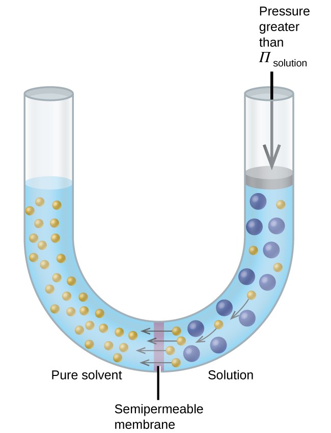
If a solution is placed in an apparatus like the one shown in Figure 12.5.5, applying pressure greater than the osmotic pressure of the solution reverses the osmosis and pushes solvent molecules from the solution into the pure solvent. This technique of reverse osmosis is used for large-scale desalination of seawater and on smaller scales to produce high-purity tap water for drinking.
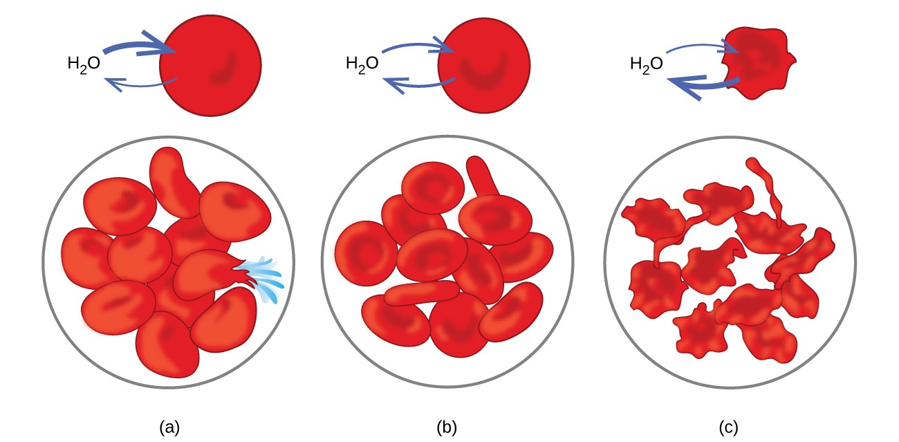
Examples of osmosis are evident in many biological systems because cells are surrounded by semipermeable membranes. Carrots and celery that have become limp because they have lost water can be made crisp again by placing them in water. Water moves into the carrot or celery cells by osmosis. A cucumber placed in a concentrated salt solution loses water by osmosis and absorbs some salt to become a pickle. Osmosis can also affect animal cells. Solute concentrations are particularly important when solutions are injected into the body. Solutes in body cell fluids and blood serum give these solutions an osmotic pressure of approximately 7.7 atm. Solutions injected into the body must have the same osmotic pressure as blood serum; that is, they should be isotonic with blood serum. If a less concentrated solution, a hypotonic solution, is injected in sufficient quantity to dilute the blood serum, water from the diluted serum passes into the blood cells by osmosis, causing the cells to expand and rupture. This process is called hemolysis. When a more concentrated solution, a hypertonic solution, is injected, the cells lose water to the more concentrated solution, shrivel, and possibly die in a process called crenation. These effects are illustrated in Figure 12.5.6.
Determination of Molar Masses
Osmotic pressure and changes in freezing point, boiling point, and vapor pressure are directly proportional to the concentration of solute present. Consequently, we can use a measurement of one of these properties to determine the molar mass of the solute from the measurements.
Example 12.5.5: Determination of a Molar Mass from a Freezing Point Depression
A solution of 4.00 g of a nonelectrolyte dissolved in 55.0 g of benzene is found to freeze at 2.32 °C. What is the molar mass of this compound?
Show Solution
We can solve this problem using the following steps.

- Determine the change in freezing point from the observed freezing point and the freezing point of pure benzene (Table 1): [latex]\Delta{T}_{\text{f}}=5.5^{\circ}\text{C}-2.32^{\circ}\text{C}=3.2^{\circ}\text{C}[/latex]
- Determine the molal concentration from Kf, the freezing point depression constant for benzene (Table 1), and ΔTf: [latex]\begin{array}{rll}\Delta{T}_{\text{f}}&=&{K}_{\text{f}}m\\ m&=&\dfrac{\Delta{T}_{\text{f}}}{{K}_{\text{f}}}=\dfrac{3.2^{\circ}\text{C}}{5.12^{\circ}\text{C}{m}^{-1}}=0.63m\end{array}[/latex]
- Determine the number of moles of compound in the solution from the molal concentration and the mass of solvent used to make the solution: [latex]\text{Moles of solute}=\dfrac{0.62\text{mol solute}}{1.00\cancel{\text{kg solvent}}}\times 0.0550\cancel{\text{kg solvent}}=0.035\text{mol}[/latex]
- Determine the molar mass from the mass of the solute and the number of moles in that mass: [latex]\text{Molar mass}=\dfrac{4.00\text{g}}{0.034\text{mol}}=1.2\times {10}^{2}\text{g/mol}[/latex]
Check Your Learning
Example 12.5.6: Determination of a Molar Mass from Osmotic Pressure
A 0.500 L sample of an aqueous solution containing 10.0 g of hemoglobin has an osmotic pressure of 5.9 torr at 22 °C. What is the molar mass of hemoglobin?
Show Solution
Here is one set of steps that can be used to solve the problem:

- Convert the osmotic pressure to atmospheres, then determine the molar concentration from the osmotic pressure: [latex]\begin{array}{l}\\ \Pi =\dfrac{5.9\text{torr}\times 1\text{atm}}{760\text{torr}}=7.8\times {10}^{-3}\text{atm}\\ \Pi =\mathit{\text{MRT}}\\ \\ M=\dfrac{\Pi }{RT}=\dfrac{7.8\times {10}^{-3}\text{atm}}{\left(0.08206\text{L atm/mol K}\right)\left(295\text{K}\right)}=3.2\times {10}^{-4}\text{M}\end{array}[/latex]
- Determine the number of moles of hemoglobin in the solution from the concentration and the volume of the solution: [latex]\text{moles of hemoglobin}=\dfrac{3.2\times {10}^{-4}\text{mol}}{1\cancel{\text{L solution}}}\times 0.500\cancel{\text{L solution}}=1.6\times {10}^{-4}\text{mol}[/latex]
- Determine the molar mass from the mass of hemoglobin and the number of moles in that mass: [latex]\text{molar mass}=\dfrac{10.0\text{g}}{1.6\times {10}^{-4}\text{mol}}=6.2\times {10}^{4}\text{g/mol}[/latex]
Check Your Learning
Key Concepts and Summary
Properties of a solution that depend only on the concentration of solute particles are called colligative properties. They include changes in the vapor pressure, boiling point, and freezing point of the solvent in the solution. The magnitudes of these properties depend only on the total concentration of solute particles in solution, not on the type of particles. The total concentration of solute particles in a solution also determines its osmotic pressure. This is the pressure that must be applied to the solution to prevent diffusion of molecules of pure solvent through a semipermeable membrane into the solution.
Key Equations
- [latex]\left({P}_{\text{A}}={X}_{\text{A}}{P}_{\text{A}}^{\circ}\right)[/latex]
- [latex]{P}_{\text{solution}}=\sum _{i}{P}_{i}=\sum _{i}{X}_{i}{P}_{i}^{\star}[/latex]
- [latex]{P}_{\text{solution}}={X}_{\text{solvent}}{P}_{\text{solvent}}^{\star}[/latex]
- [latex]\Delta{T}_{\text{b}}={K}_{\text{b}}m[/latex]
- [latex]\Delta{T}_{\text{f}}={K}_{\text{f}}m[/latex]
- [latex]\Pi =MRT[/latex]
Try It
- A solution contains 5.00 g of urea, [latex]\ce{CO(NH2)2}[/latex], a nonvolatile compound, dissolved in 0.100 kg of water. If the vapor pressure of pure water at 25 °C is 23.7 torr, what is the vapor pressure of the solution?
- What is the molar mass of a solution of 5.00 g of a compound in 25.00 g of carbon tetrachloride (bp 76.8 °C; Kb = 5.02 °C/m) that boils at 81.5 °C at 1 atm?
- Outline the steps necessary to answer the question.
- Solve the problem.
- What is the boiling point of a solution of 115.0 g of sucrose, [latex]\ce{C_{12}H_{22}O_{11}}[/latex], in 350.0 g of water?
- Outline the steps necessary to answer the question
- Answer the question
- What is the freezing temperature of a solution of 115.0 g of sucrose, [latex]\ce{C_{12}H_{22}O_{11}}[/latex], in 350.0 g of water, which freezes at 0.0 °C when pure?
- Outline the steps necessary to answer the question.
- Answer the question.
5. What is the osmotic pressure of an aqueous solution of 1.64 g of [latex]\ce{Ca(NO3)2}[/latex] in water at 25 °C? The volume of the solution is 275 mL.
-
- Outline the steps necessary to answer the question.
- Answer the question.
Show Selected Solutions
2. The molar mass of a solution of 5.00 g of a compound in 25.00 g of carbon tetrachloride (bp 76.8 °C; Kb = 5.02 °C/m) can be found as follows:
- Determine the molal concentration from the change in boiling point and Kb; determine the moles of solute in the solution from the molal concentration and mass of solvent; determine the molar mass from the number of moles and the mass of solute.
- [latex]\Delta[/latex]Tb = 81.5 − 76.8 = 4.7 °C, [latex]\Delta[/latex]Tb = Kbm, so [latex]m=\frac{\Delta{T}_{\text{b}}}{{K}_{\text{b}}}=\frac{4.7^{\circ}\text{C}}{5.02^{\circ}\text{C/}m}=0.94m[/latex]. Moles of solute = molality × kg of solvent = 0.94 m 0.02500 kg = 0.024 mol;
[latex]\text{molar mass}=\frac{\text{mass}}{\text{moles}}=\frac{5.00\text{g}}{0.024\text{mol}}=2.1\times {10}^{2}\text{g}{\text{mol}}^{-1}[/latex]
Molecular mass = 2.1 × 10² g mol−1
3. The boiling point can be found as follows:
- Determine the molar mass of sucrose; determine the number of moles of sucrose in the solution; convert the mass of solvent to units of kilograms; from the number of moles and the mass of solvent, determine the molality; determine the difference between the boiling point of water and the boiling point of the solution; determine the new boiling point.
- [latex]\begin{array}{l}{ }\text{mol sucrose}=\frac{115.0\text{g}}{342.300\text{g}{\text{mol}}^{-1}}=0.3360\text{mol}\\ \text{molality}=\frac{0.3360\text{mol}{\ce{C}}_{\ce{12}}{\ce{H}}_{\ce{22}}{\ce{O}}_{\ce{11}}}{0.3500\text{kg}{\ce{H}}_{\ce{2}}\ce{O}}=0.9599m\end{array}[/latex]
ΔTb = Kbm = (0.512 °C m–1)(0.9599 m) = 0.491 °C
The boiling point of pure water at 100.0 °C increases 0.491 °C to 100.491 °C, or 100.5 °C.
4. The freezing temperature can be found as follows:
- Determine the molar mass of sucrose; determine the number of moles of sucrose in the solution; convert the mass of solvent to units of kilograms; from the number of moles and the mass of solvent, determine the molality; determine the difference between the freezing temperature of water and the freezing temperature of the solution; determine the new freezing temperature.
- [latex]\begin{array}{l} \text{mol sucrose}=\frac{115.0\text{g}}{342.300\text{g}{\text{mol}}^{-1}}=0.336\text{mol}\\ m\text{ sucrose}=\frac{0.336\text{mol}}{0.350\text{kg}}=0.960m\end{array}[/latex]
ΔTb = Kbm = (1.86 °C m–1)(0.960 m) = 1.78 °C
The freezing temperature is 0.0 °C – 1.78 °C = –1.8 °C.
5. The osmotic pressure of an aqueous solution of 1.64 g of [latex]\ce{Ca(NO3)2}[/latex] in water at 25 °C can be found as follows:
- Determine the molar mass of [latex]\ce{Ca(NO3)2}[/latex]; determine the number of moles of [latex]\ce{Ca(NO3)2}[/latex] in the solution; determine the number of moles of ions in the solution; determine the molarity of ions, then the osmotic pressure.
- [latex]M\ce{Ca}{\left({\ce{NO}}_{3}\right)}_{2}=\dfrac{1.64\text{g } \ce{Ca}{\left({\ce{NO}}_{3}\right)}_{2}\times 1\text{mol/}164.088\text{g } \ce{Ca}{\left({\ce{NO}}_{3}\right)}_{2}}{0.275\text{L}}=0.363\text{M}[/latex]
The molarity of the ions is three times the molarity of [latex]\ce{Ca(NO3)2}[/latex]. Therefore, multiply the molarity of [latex]\ce{Ca(NO3)2}[/latex] by 3: [latex]\Pi[/latex] = MRT = 3 × 0.0363 mol L–1 × 0.08206 L atm mol–1 K–1 × 298.15 K = 2.67 atm.
Glossary
boiling point elevation: elevation of the boiling point of a liquid by addition of a solute
boiling point elevation constant: the proportionality constant in the equation relating boiling point elevation to solute molality; also known as the ebullioscopic constant
colligative property: property of a solution that depends only on the concentration of a solute species
crenation: process whereby biological cells become shriveled due to loss of water by osmosis
freezing point depression: lowering of the freezing point of a liquid by addition of a solute
freezing point depression constant: (also, cryoscopic constant) proportionality constant in the equation relating freezing point depression to solute molality
hemolysis: rupture of red blood cells due to the accumulation of excess water by osmosis
hypertonic: of greater osmotic pressure
hypotonic: of less osmotic pressure
ion pair: solvated anion/cation pair held together by moderate electrostatic attraction
isotonic: of equal osmotic pressure
osmosis: diffusion of solvent molecules through a semipermeable membrane
osmotic pressure (Π): opposing pressure required to prevent bulk transfer of solvent molecules through a semipermeable membrane
Raoult’s law: the partial pressure exerted by a solution component is equal to the product of the component’s mole fraction in the solution and its equilibrium vapor pressure in the pure state
semipermeable membrane: a membrane that selectively permits passage of certain ions or molecules
Licenses and Attributions (Click to expand)
CC licensed content, Shared previously
- Chemistry 2e. Provided by: OpenStax. Located at: https://openstax.org/. License: CC BY: Attribution. License Terms: Access for free at
https://openstax.org/books/chemistry-2e/pages/1-introduction
property of a solution that depends only on the concentration of a solute species
the partial pressure exerted by a solution component is equal to the product of the component’s mole fraction in the solution and its equilibrium vapor pressure in the pure state
elevation of the boiling point of a liquid by addition of a solute
the proportionality constant in the equation relating boiling point elevation to solute molality; also known as the ebullioscopic constant
lowering of the freezing point of a liquid by addition of a solute
(also, cryoscopic constant) proportionality constant in the equation relating freezing point depression to solute molality
a membrane that selectively permits passage of certain ions or molecules
diffusion of solvent molecules through a semipermeable membrane
opposing pressure required to prevent bulk transfer of solvent molecules through a semipermeable membrane
of equal osmotic pressure
of less osmotic pressure
rupture of red blood cells due to the accumulation of excess water by osmosis
of greater osmotic pressure
process whereby biological cells become shriveled due to loss of water by osmosis
