7.4 Determining Field from Potential

Recall that we were able, in certain systems, to calculate the potential by integrating over the electric field. As you may already suspect, this means that we may calculate the electric field by taking derivatives of the potential, although going from a scalar to a vector quantity introduces some interesting wrinkles. We frequently need [latex]\stackrel{\to }{\textbf{E}}[/latex] to calculate the force in a system; since it is often simpler to calculate the potential directly, there are systems in which it is useful to calculate V and then derive [latex]\stackrel{\to }{\textbf{E}}[/latex] from it.

In general, regardless of whether the electric field is uniform, it points in the direction of decreasing potential, because the force on a positive charge is in the direction of [latex]\stackrel{\to }{\textbf{E}}[/latex] and also in the direction of lower potential V. Furthermore, the magnitude of [latex]\stackrel{\to }{\textbf{E}}[/latex] equals the rate of decrease of V with distance. The faster V decreases over distance, the greater the electric field. This gives us the following result.

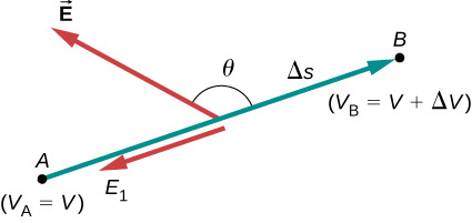
For continually changing potentials, [latex]\text{Δ}V[/latex] and [latex]\text{Δ}s[/latex] become infinitesimals, and we need differential calculus to determine the electric field. As shown in Figure 7.27, if we treat the distance [latex]\text{Δ}s[/latex] as very small so that the electric field is essentially constant over it, we find that

Therefore, the electric field components in the Cartesian directions are given by

This allows us to define the “grad” or “del” vector operator, which allows us to compute the gradient in one step. In Cartesian coordinates, it takes the form

With this notation, we can calculate the electric field from the potential with

a process we call calculating the gradient of the potential.

If we have a system with either cylindrical or spherical symmetry, we only need to use the del operator in the appropriate coordinates:

Example

Electric Field of a Point Charge

Calculate the electric field of a point charge from the potential.

Strategy

The potential is known to be [latex]V=k\frac{q}{r}[/latex], which has a spherical symmetry. Therefore, we use the spherical del operator in the formula [latex]\stackrel{\to }{\textbf{E}}=\text{−}\stackrel{\to }{\nabla }V[/latex].

Solution

Show Answer

Performing this calculation gives us

[latex]\stackrel{\to }{\textbf{E}}=\text{−}\left(\hat{\textbf{r}}\frac{\partial }{\partial r}+\hat{\mathit{\textbf{θ}}}\frac{1}{r}\phantom{\rule{0.2em}{0ex}}\frac{\partial }{\partial \theta }+\hat{\mathit{\textbf{φ}}}\frac{1}{r\phantom{\rule{0.2em}{0ex}}\text{sin}\phantom{\rule{0.2em}{0ex}}\theta }\phantom{\rule{0.2em}{0ex}}\frac{\partial }{\partial \phi }\right)k\frac{q}{r}=\text{−}kq\left(\hat{\textbf{r}}\frac{\partial }{\partial r}\phantom{\rule{0.2em}{0ex}}\frac{1}{r}+\hat{\mathit{\textbf{θ}}}\frac{1}{r}\phantom{\rule{0.2em}{0ex}}\frac{\partial }{\partial \theta }\phantom{\rule{0.2em}{0ex}}\frac{1}{r}+\hat{\mathit{\textbf{φ}}}\frac{1}{r\phantom{\rule{0.2em}{0ex}}\text{sin}\phantom{\rule{0.2em}{0ex}}\theta }\phantom{\rule{0.2em}{0ex}}\frac{\partial }{\partial \phi }\phantom{\rule{0.2em}{0ex}}\frac{1}{r}\right).[/latex]

This equation simplifies to

[latex]\stackrel{\to }{\textbf{E}}=\text{−}kq\left(\hat{\textbf{r}}\frac{-1}{{r}^{2}}+\hat{\mathit{\textbf{θ}}}0+\hat{\mathit{\textbf{φ}}}0\right)=k\frac{q}{{r}^{2}}\hat{\textbf{r}}[/latex]

as expected.

Significance

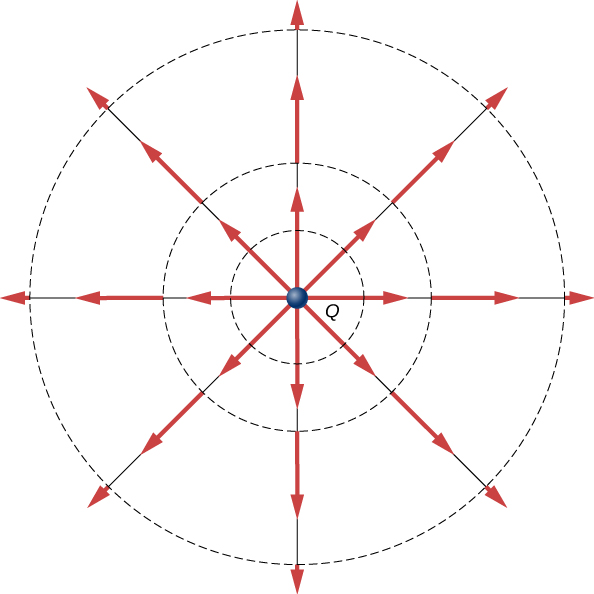
We not only obtained the equation for the electric field of a point particle that we’ve seen before, we also have a demonstration that [latex]\stackrel{\to }{\textbf{E}}[/latex] points in the direction of decreasing potential, as shown in Figure 7.28.

Example

Electric Field of a Ring of Charge

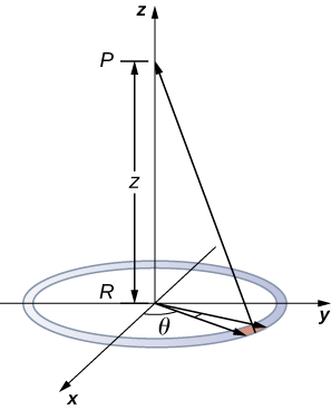
Use the potential found in Example 7.8 to calculate the electric field along the axis of a ring of charge (Figure 7.29).

Strategy

In this case, we are only interested in one dimension, the z-axis. Therefore, we use [latex]{E}_{z}=-\frac{\partial V}{\partial z}[/latex]

with the potential [latex]V=k\frac{{q}_{\text{tot}}}{\sqrt{{z}^{2}+{R}^{2}}}[/latex] found previously.

Solution

Show Answer

Taking the derivative of the potential yields

[latex]{E}_{z}=-\frac{\partial }{\partial z}\phantom{\rule{0.2em}{0ex}}\frac{k{q}_{\text{tot}}}{\sqrt{{z}^{2}+{R}^{2}}}=k\frac{{q}_{\text{tot}}z}{{\left({z}^{2}+{R}^{2}\right)}^{3\text{/}2}}.[/latex]

Significance

Again, this matches the equation for the electric field found previously. It also demonstrates a system in which using the full del operator is not necessary.