
Chapter 7. Electric Potential
7.5 Equipotential Surfaces and Conductors
Learning Objectives
By the end of this section, you will be able to:
- Define equipotential surfaces and equipotential lines
- Explain the relationship between equipotential lines and electric field lines
- Map equipotential lines for one or two point charges
- Describe the potential of a conductor
- Compare and contrast equipotential lines and elevation lines on topographic maps
We can represent electric potentials (voltages) pictorially, just as we drew pictures to illustrate electric fields. This is not surprising, since the two concepts are related. Consider Figure 7.30, which shows an isolated positive point charge and its electric field lines, which radiate out from a positive charge and terminate on negative charges. We use red arrows to represent the magnitude and direction of the electric field, and we use black lines to represent places where the electric potential is constant. These are called equipotential surfaces in three dimensions, or equipotential lines in two dimensions. The term equipotential is also used as a noun, referring to an equipotential line or surface. The potential for a point charge is the same anywhere on an imaginary sphere of radius r surrounding the charge. This is true because the potential for a point charge is given by [latex]V=kq\text{/}r[/latex] and thus has the same value at any point that is a given distance r from the charge. An equipotential sphere is a circle in the two-dimensional view of Figure 7.30. Because the electric field lines point radially away from the charge, they are perpendicular to the equipotential lines.
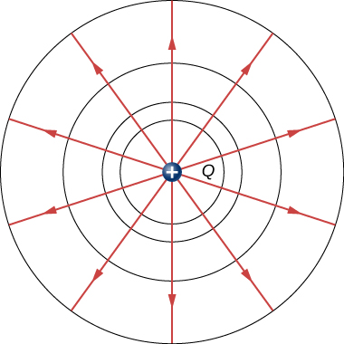
It is important to note that equipotential lines are always perpendicular to electric field lines. No work is required to move a charge along an equipotential, since [latex]\text{Δ}V=0[/latex]. Thus, the work is
Work is zero if the direction of the force is perpendicular to the displacement. Force is in the same direction as E, so motion along an equipotential must be perpendicular to E. More precisely, work is related to the electric field by
Note that in this equation, E and F symbolize the magnitudes of the electric field and force, respectively. Neither q nor E is zero; d is also not zero. So [latex]\text{cos}\phantom{\rule{0.2em}{0ex}}\theta[/latex] must be 0, meaning [latex]\theta[/latex] must be [latex]90\text{º}[/latex]. In other words, motion along an equipotential is perpendicular to E.
One of the rules for static electric fields and conductors is that the electric field must be perpendicular to the surface of any conductor. This implies that a conductor is an equipotential surface in static situations. There can be no voltage difference across the surface of a conductor, or charges will flow. One of the uses of this fact is that a conductor can be fixed at what we consider zero volts by connecting it to the earth with a good conductor—a process called grounding. Grounding can be a useful safety tool. For example, grounding the metal case of an electrical appliance ensures that it is at zero volts relative to Earth.
Because a conductor is an equipotential, it can replace any equipotential surface. For example, in Figure 7.30, a charged spherical conductor can replace the point charge, and the electric field and potential surfaces outside of it will be unchanged, confirming the contention that a spherical charge distribution is equivalent to a point charge at its center.
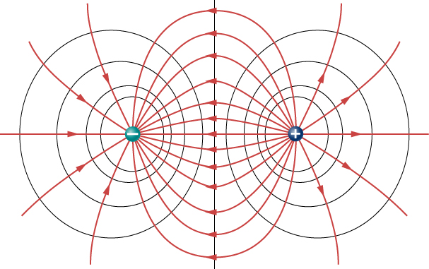
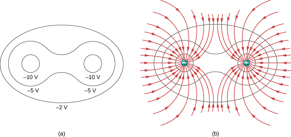
Figure 7.31 shows the electric field and equipotential lines for two equal and opposite charges. Given the electric field lines, the equipotential lines can be drawn simply by making them perpendicular to the electric field lines. Conversely, given the equipotential lines, as in Figure 7.32(a), the electric field lines can be drawn by making them perpendicular to the equipotentials, as in Figure 7.32(b).
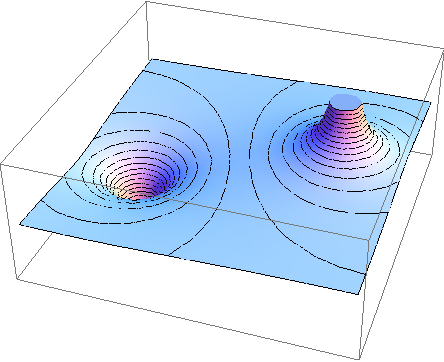
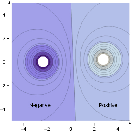
To improve your intuition, we show a three-dimensional variant of the potential in a system with two opposing charges. Figure 7.33 displays a three-dimensional map of electric potential, where lines on the map are for equipotential surfaces. The hill is at the positive charge, and the trough is at the negative charge. The potential is zero far away from the charges. Note that the cut off at a particular potential implies that the charges are on conducting spheres with a finite radius.
A two-dimensional map of the cross-sectional plane that contains both charges is shown in Figure 7.34. The line that is equidistant from the two opposite charges corresponds to zero potential, since at the points on the line, the positive potential from the positive charge cancels the negative potential from the negative charge. Equipotential lines in the cross-sectional plane are closed loops, which are not necessarily circles, since at each point, the net potential is the sum of the potentials from each charge.
View this simulation to observe and modify the equipotential surfaces and electric fields for many standard charge configurations. There’s a lot to explore.
One of the most important cases is that of the familiar parallel conducting plates shown in Figure 7.35. Between the plates, the equipotentials are evenly spaced and parallel. The same field could be maintained by placing conducting plates at the equipotential lines at the potentials shown.
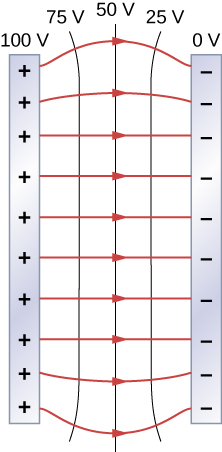
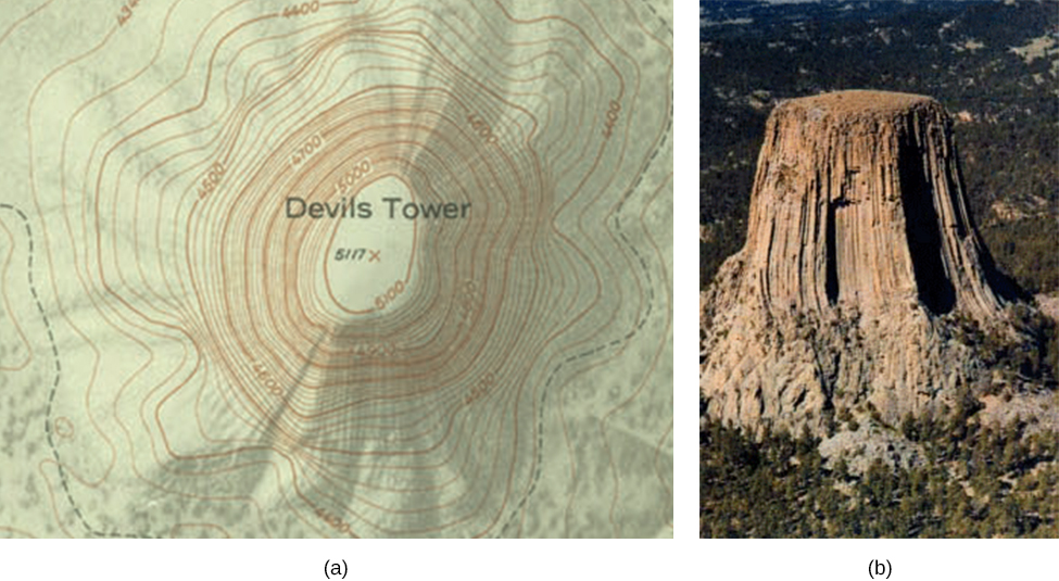
Consider the parallel plates in Figure 7.2. These have equipotential lines that are parallel to the plates in the space between and evenly spaced. An example of this (with sample values) is given in Figure 7.35. We could draw a similar set of equipotential isolines for gravity on the hill shown in Figure 7.2. If the hill has any extent at the same slope, the isolines along that extent would be parallel to each other. Furthermore, in regions of constant slope, the isolines would be evenly spaced. An example of real topographic lines is shown in Figure 7.36.
Example
Calculating Equipotential Lines
You have seen the equipotential lines of a point charge in Figure 7.30. How do we calculate them? For example, if we have a [latex]\text{+}10\text{-nC}[/latex] charge at the origin, what are the equipotential surfaces at which the potential is (a) 100 V, (b) 50 V, (c) 20 V, and (d) 10 V?
Strategy
Set the equation for the potential of a point charge equal to a constant and solve for the remaining variable(s). Then calculate values as needed.
Solution
Show Answer
In [latex]V=k\frac{q}{r}[/latex], let V be a constant. The only remaining variable is r; hence, [latex]r=k\frac{q}{V}=\text{constant}[/latex]. Thus, the equipotential surfaces are spheres about the origin. Their locations are:
- [latex]r=k\frac{q}{V}=\left(8.99\phantom{\rule{0.2em}{0ex}}×\phantom{\rule{0.2em}{0ex}}{10}^{9}\phantom{\rule{0.2em}{0ex}}{\text{Nm}}^{2}{\text{/C}}^{2}\right)\frac{\left(10\phantom{\rule{0.2em}{0ex}}×\phantom{\rule{0.2em}{0ex}}{10}^{-9}\phantom{\rule{0.2em}{0ex}}\text{C}\right)}{100\phantom{\rule{0.2em}{0ex}}\text{V}}=0.90\phantom{\rule{0.2em}{0ex}}\text{m}[/latex];
- [latex]r=k\frac{q}{V}=\left(8.99\phantom{\rule{0.2em}{0ex}}×\phantom{\rule{0.2em}{0ex}}{10}^{9}\phantom{\rule{0.2em}{0ex}}{\text{Nm}}^{2}{\text{/C}}^{2}\right)\frac{\left(10\phantom{\rule{0.2em}{0ex}}×\phantom{\rule{0.2em}{0ex}}{10}^{-9}\phantom{\rule{0.2em}{0ex}}\text{C}\right)}{50\phantom{\rule{0.2em}{0ex}}\text{V}}=1.8\phantom{\rule{0.2em}{0ex}}\text{m}[/latex];
- [latex]r=k\frac{q}{V}=\left(8.99\phantom{\rule{0.2em}{0ex}}×\phantom{\rule{0.2em}{0ex}}{10}^{9}\phantom{\rule{0.2em}{0ex}}{\text{Nm}}^{2}{\text{/C}}^{2}\right)\frac{\left(10\phantom{\rule{0.2em}{0ex}}×\phantom{\rule{0.2em}{0ex}}{10}^{-9}\phantom{\rule{0.2em}{0ex}}\text{C}\right)}{20\phantom{\rule{0.2em}{0ex}}\text{V}}=4.5\phantom{\rule{0.2em}{0ex}}\text{m}[/latex];
- [latex]r=k\frac{q}{V}=\left(8.99\phantom{\rule{0.2em}{0ex}}×\phantom{\rule{0.2em}{0ex}}{10}^{9}\phantom{\rule{0.2em}{0ex}}{\text{Nm}}^{2}{\text{/C}}^{2}\right)\frac{\left(10\phantom{\rule{0.2em}{0ex}}×\phantom{\rule{0.2em}{0ex}}{10}^{-9}\phantom{\rule{0.2em}{0ex}}\text{C}\right)}{10\phantom{\rule{0.2em}{0ex}}\text{V}}=9.0\phantom{\rule{0.2em}{0ex}}\text{m}[/latex].
Significance
This means that equipotential surfaces around a point charge are spheres of constant radius, as shown earlier, with well-defined locations.
Example
Potential Difference between Oppositely Charged Parallel Plates
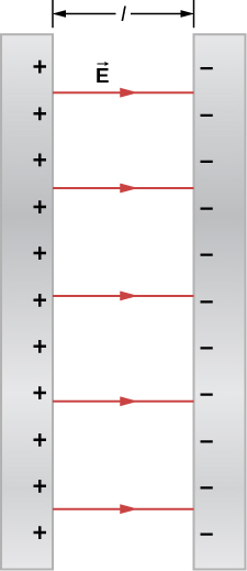
Two large conducting plates carry equal and opposite charges, with a surface charge density [latex]\sigma[/latex] of magnitude [latex]6.81\phantom{\rule{0.2em}{0ex}}×\phantom{\rule{0.2em}{0ex}}{10}^{-7}\phantom{\rule{0.2em}{0ex}}{\text{C/m}}^{2},[/latex] as shown in Figure 7.37. The separation between the plates is [latex]l=6.50\phantom{\rule{0.2em}{0ex}}\text{mm}[/latex]. (a) What is the electric field between the plates? (b) What is the potential difference between the plates? (c) What is the distance between equipotential planes which differ by 100 V?
Strategy
(a) Since the plates are described as “large” and the distance between them is not, we will approximate each of them as an infinite plane, and apply the result from Gauss’s law in the previous chapter.
(b) Use [latex]\text{Δ}{V}_{AB}=\text{−}{\int }_{A}^{B}\stackrel{\to }{\textbf{E}}·d\stackrel{\to }{\textbf{l}}[/latex].
(c) Since the electric field is constant, find the ratio of 100 V to the total potential difference; then calculate this fraction of the distance.
Solution
Show Answer
- The electric field is directed from the positive to the negative plate as shown in the figure, and its magnitude is given by
[latex]E=\frac{\sigma }{{\epsilon }_{0}}=\frac{6.81\phantom{\rule{0.2em}{0ex}}×\phantom{\rule{0.2em}{0ex}}{10}^{-7}\phantom{\rule{0.2em}{0ex}}{\text{C/m}}^{2}}{8.85\phantom{\rule{0.2em}{0ex}}×\phantom{\rule{0.2em}{0ex}}{10}^{-12}\phantom{\rule{0.2em}{0ex}}{\text{C}}^{2}\text{/}\text{N}·{\text{m}}^{2}}=7.69\phantom{\rule{0.2em}{0ex}}×\phantom{\rule{0.2em}{0ex}}{10}^{4}\phantom{\rule{0.2em}{0ex}}\text{V/m}\text{.}[/latex] - To find the potential difference [latex]\text{Δ}V[/latex] between the plates, we use a path from the negative to the positive plate that is directed against the field. The displacement vector [latex]d\stackrel{\to }{\textbf{l}}[/latex] and the electric field [latex]\stackrel{\to }{\textbf{E}}[/latex] are antiparallel so [latex]\stackrel{\to }{\textbf{E}}·d\stackrel{\to }{\textbf{l}}=\text{−}E\phantom{\rule{0.2em}{0ex}}dl.[/latex] The potential difference between the positive plate and the negative plate is then
[latex]\text{Δ}V=\text{−}\int E·dl=E\int dl=El=\left(7.69\phantom{\rule{0.2em}{0ex}}×\phantom{\rule{0.2em}{0ex}}{10}^{4}\phantom{\rule{0.2em}{0ex}}\text{V/m}\right)\left(6.50\phantom{\rule{0.2em}{0ex}}×\phantom{\rule{0.2em}{0ex}}{10}^{-3}\phantom{\rule{0.2em}{0ex}}\text{m}\right)=500\phantom{\rule{0.2em}{0ex}}\text{V}\text{.}[/latex] - The total potential difference is 500 V, so 1/5 of the distance between the plates will be the distance between 100-V potential differences. The distance between the plates is 6.5 mm, so there will be 1.3 mm between 100-V potential differences.
Significance
You have now seen a numerical calculation of the locations of equipotentials between two charged parallel plates.
Check Your Understanding
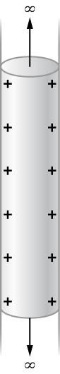
What are the equipotential surfaces for an infinite line charge?
Show Solution
infinite cylinders of constant radius, with the line charge as the axis
Distribution of Charges on Conductors
In Example 7.19 with a point charge, we found that the equipotential surfaces were in the form of spheres, with the point charge at the center. Given that a conducting sphere in electrostatic equilibrium is a spherical equipotential surface, we should expect that we could replace one of the surfaces in Example 7.19 with a conducting sphere and have an identical solution outside the sphere. Inside will be rather different, however.
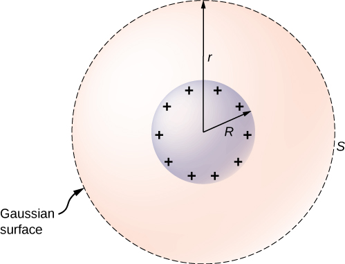
To investigate this, consider the isolated conducting sphere of Figure 7.38 that has a radius R and an excess charge q. To find the electric field both inside and outside the sphere, note that the sphere is isolated, so its surface change distribution and the electric field of that distribution are spherically symmetric. We can therefore represent the field as [latex]\stackrel{\to }{\textbf{E}}=E\left(r\right)\hat{\textbf{r}}.[/latex] To calculate E(r), we apply Gauss’s law over a closed spherical surface S of radius r that is concentric with the conducting sphere. Since r is constant and [latex]\hat{\textbf{n}}=\hat{\textbf{r}}[/latex] on the sphere,
For [latex]r\phantom{\rule{0.2em}{0ex}}< \phantom{\rule{0.2em}{0ex}}R[/latex], S is within the conductor, so recall from our previous study of Gauss’s law that [latex]{q}_{\text{enc}}=0[/latex] and Gauss’s law gives [latex]E\left(r\right)=0[/latex], as expected inside a conductor at equilibrium. If [latex]r\phantom{\rule{0.2em}{0ex}}>\phantom{\rule{0.2em}{0ex}}R[/latex], S encloses the conductor so [latex]{q}_{\text{enc}}=q.[/latex] From Gauss’s law,
The electric field of the sphere may therefore be written as
As expected, in the region [latex]r\ge R,[/latex] the electric field due to a charge q placed on an isolated conducting sphere of radius R is identical to the electric field of a point charge q located at the center of the sphere.
To find the electric potential inside and outside the sphere, note that for [latex]r\ge R,[/latex] the potential must be the same as that of an isolated point charge q located at [latex]r=0[/latex],
simply due to the similarity of the electric field.
For [latex]rV(r) is constant in this region. Since [latex]V\left(R\right)=q\text{/}4\pi {\epsilon }_{0}R,[/latex]
We will use this result to show that
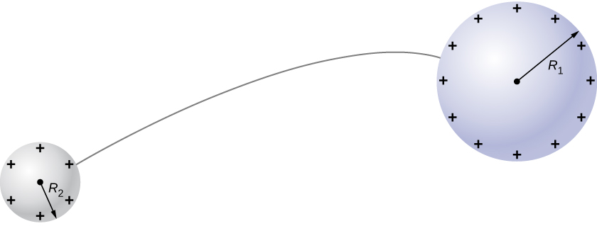
for two conducting spheres of radii [latex]{R}_{1}\phantom{\rule{0.2em}{0ex}}\text{and}\phantom{\rule{0.2em}{0ex}}{R}_{2}[/latex], with surface charge densities [latex]{\sigma }_{1}\phantom{\rule{0.2em}{0ex}}\text{and}\phantom{\rule{0.2em}{0ex}}{\sigma }_{2}[/latex] respectively, that are connected by a thin wire, as shown in Figure 7.39. The spheres are sufficiently separated so that each can be treated as if it were isolated (aside from the wire). Note that the connection by the wire means that this entire system must be an equipotential.
We have just seen that the electrical potential at the surface of an isolated, charged conducting sphere of radius R is
Now, the spheres are connected by a conductor and are therefore at the same potential; hence
and
The net charge on a conducting sphere and its surface charge density are related by [latex]q=\sigma \left(4\pi {R}^{2}\right).[/latex] Substituting this equation into the previous one, we find
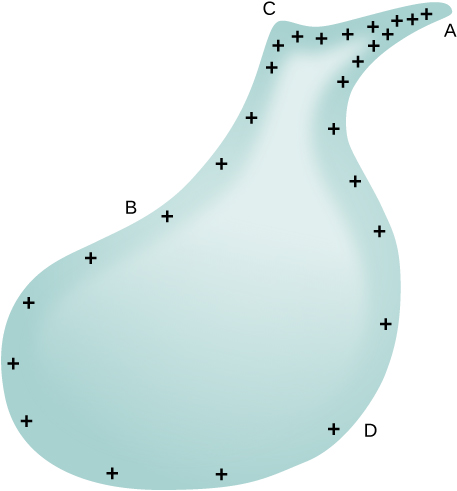
Obviously, two spheres connected by a thin wire do not constitute a typical conductor with a variable radius of curvature. Nevertheless, this result does at least provide a qualitative idea of how charge density varies over the surface of a conductor. The equation indicates that where the radius of curvature is large (points B and D in Figure 7.40), [latex]\sigma[/latex] and E are small.
Similarly, the charges tend to be denser where the curvature of the surface is greater, as demonstrated by the charge distribution on oddly shaped metal (Figure 7.40). The surface charge density is higher at locations with a small radius of curvature than at locations with a large radius of curvature.
A practical application of this phenomenon is the lightning rod, which is simply a grounded metal rod with a sharp end pointing upward. As positive charge accumulates in the ground due to a negatively charged cloud overhead, the electric field around the sharp point gets very large. When the field reaches a value of approximately [latex]3.0\phantom{\rule{0.2em}{0ex}}×\phantom{\rule{0.2em}{0ex}}{10}^{6}\phantom{\rule{0.2em}{0ex}}\text{N/C}[/latex] (the dielectric strength of the air), the free ions in the air are accelerated to such high energies that their collisions with air molecules actually ionize the molecules. The resulting free electrons in the air then flow through the rod to Earth, thereby neutralizing some of the positive charge. This keeps the electric field between the cloud and the ground from getting large enough to produce a lightning bolt in the region around the rod.
An important application of electric fields and equipotential lines involves the heart. The heart relies on electrical signals to maintain its rhythm. The movement of electrical signals causes the chambers of the heart to contract and relax. When a person has a heart attack, the movement of these electrical signals may be disturbed. An artificial pacemaker and a defibrillator can be used to initiate the rhythm of electrical signals. The equipotential lines around the heart, the thoracic region, and the axis of the heart are useful ways of monitoring the structure and functions of the heart. An electrocardiogram (ECG) measures the small electric signals being generated during the activity of the heart.
Play around with this simulation to move point charges around on the playing field and then view the electric field, voltages, equipotential lines, and more.
Summary
- An equipotential surface is the collection of points in space that are all at the same potential. Equipotential lines are the two-dimensional representation of equipotential surfaces.
- Equipotential surfaces are always perpendicular to electric field lines.
- Conductors in static equilibrium are equipotential surfaces.
- Topographic maps may be thought of as showing gravitational equipotential lines.
Conceptual Questions
If two points are at the same potential, are there any electric field lines connecting them?
Show Solution
no
Suppose you have a map of equipotential surfaces spaced 1.0 V apart. What do the distances between the surfaces in a particular region tell you about the strength of the [latex]\stackrel{\to }{\textbf{E}}[/latex] in that region?
Is the electric potential necessarily constant over the surface of a conductor?
Show Solution
No; it might not be at electrostatic equilibrium.
Under electrostatic conditions, the excess charge on a conductor resides on its surface. Does this mean that all of the conduction electrons in a conductor are on the surface?
Can a positively charged conductor be at a negative potential? Explain.
Show Solution
Yes. It depends on where the zero reference for potential is. (Though this might be unusual.)
Can equipotential surfaces intersect?
Problems
Two very large metal plates are placed 2.0 cm apart, with a potential difference of 12 V between them. Consider one plate to be at 12 V, and the other at 0 V. (a) Sketch the equipotential surfaces for 0, 4, 8, and 12 V. (b) Next sketch in some electric field lines, and confirm that they are perpendicular to the equipotential lines.
A very large sheet of insulating material has had an excess of electrons placed on it to a surface charge density of [latex]–3.00\phantom{\rule{0.2em}{0ex}}{\text{nC/m}}^{2}[/latex]. (a) As the distance from the sheet increases, does the potential increase or decrease? Can you explain why without any calculations? Does the location of your reference point matter? (b) What is the shape of the equipotential surfaces? (c) What is the spacing between surfaces that differ by 1.00 V?
Show Solution
a. increases; the constant (negative) electric field has this effect, the reference point only matters for magnitude; b. they are planes parallel to the sheet; c. 0.006 m/V
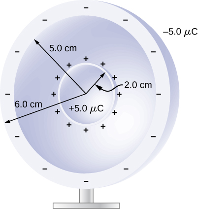
A metallic sphere of radius 2.0 cm is charged with [latex]\text{+}5.0\text{-}\mu \text{C}[/latex] charge, which spreads on the surface of the sphere uniformly. The metallic sphere stands on an insulated stand and is surrounded by a larger metallic spherical shell, of inner radius 5.0 cm and outer radius 6.0 cm. Now, a charge of [latex]-5.0\text{-}\mu \text{C}[/latex] is placed on the inside of the spherical shell, which spreads out uniformly on the inside surface of the shell. If potential is zero at infinity, what is the potential of (a) the spherical shell, (b) the sphere, (c) the space between the two, (d) inside the sphere, and (e) outside the shell?
Two large charged plates of charge density [latex]\text{±}30\phantom{\rule{0.2em}{0ex}}\mu {\text{C/m}}^{2}[/latex] face each other at a separation of 5.0 mm. (a) Find the electric potential everywhere. (b) An electron is released from rest at the negative plate; with what speed will it strike the positive plate?
Show Solution
a. from the previous chapter, the electric field has magnitude [latex]\frac{\sigma }{{\epsilon }_{0}}[/latex] in the region between the plates and zero outside; defining the negatively charged plate to be at the origin and zero potential, with the positively charged plate located at [latex]\text{+}5\phantom{\rule{0.2em}{0ex}}\text{mm}[/latex] in the z-direction, [latex]V=1.7\phantom{\rule{0.2em}{0ex}}×\phantom{\rule{0.2em}{0ex}}{10}^{4}\phantom{\rule{0.2em}{0ex}}\text{V}[/latex] so the potential is 0 for [latex]z<0,\phantom{\rule{0.2em}{0ex}}1.7\phantom{\rule{0.2em}{0ex}}×\phantom{\rule{0.2em}{0ex}}{10}^{4}\phantom{\rule{0.2em}{0ex}}\text{V}\left(\frac{z}{5\phantom{\rule{0.2em}{0ex}}\text{mm}}\right)[/latex] for [latex]0\le z\le 5\phantom{\rule{0.2em}{0ex}}\text{mm,}\phantom{\rule{0.2em}{0ex}}1.7\phantom{\rule{0.2em}{0ex}}×\phantom{\rule{0.2em}{0ex}}{10}^{4}\phantom{\rule{0.2em}{0ex}}\text{V}[/latex] for [latex]z>5\phantom{\rule{0.2em}{0ex}}\text{mm;}[/latex]
b. [latex]qV=\frac{1}{2}m{v}^{2}\to v=7.7\phantom{\rule{0.2em}{0ex}}×\phantom{\rule{0.2em}{0ex}}{10}^{7}\phantom{\rule{0.2em}{0ex}}\text{m/s}[/latex]
A long cylinder of aluminum of radius R meters is charged so that it has a uniform charge per unit length on its surface of [latex]\lambda[/latex].
(a) Find the electric field inside and outside the cylinder. (b) Find the electric potential inside and outside the cylinder. (c) Plot electric field and electric potential as a function of distance from the center of the rod.
Two parallel plates 10 cm on a side are given equal and opposite charges of magnitude [latex]5.0\phantom{\rule{0.2em}{0ex}}×\phantom{\rule{0.2em}{0ex}}{10}^{-9}\phantom{\rule{0.2em}{0ex}}\text{C}\text{.}[/latex] The plates are 1.5 mm apart. What is the potential difference between the plates?
Show Solution
[latex]V=85\phantom{\rule{0.2em}{0ex}}\text{V}[/latex]
The surface charge density on a long straight metallic pipe is [latex]\sigma[/latex]. What is the electric potential outside and inside the pipe? Assume the pipe has a diameter of 2a.
Concentric conducting spherical shells carry charges Q and –Q, respectively. The inner shell has negligible thickness. What is the potential difference between the shells?
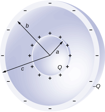
Show Solution
In the region [latex]a\le r\le b,\phantom{\rule{0.2em}{0ex}}\stackrel{\to }{\textbf{E}}=\frac{kQ}{{r}^{2}}\hat{\textbf{r}}[/latex], and E is zero elsewhere; hence, the potential difference is [latex]V=kQ\left(\frac{1}{a}-\frac{1}{b}\right)[/latex].
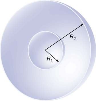
Shown below are two concentric spherical shells of negligible thicknesses and radii [latex]{R}_{1}[/latex] and [latex]{R}_{2}.[/latex] The inner and outer shell carry net charges [latex]{q}_{1}[/latex] and [latex]{q}_{2},[/latex] respectively, where both [latex]{q}_{1}[/latex] and [latex]{q}_{2}[/latex] are positive. What is the electric potential in the regions (a) [latex]r< {R}_{1},[/latex] (b) [latex]{R}_{1}< r< {R}_{2},[/latex] and (c) [latex]r>{R}_{2}?[/latex]
A solid cylindrical conductor of radius a is surrounded by a concentric cylindrical shell of inner radius b. The solid cylinder and the shell carry charges Q and –Q, respectively. Assuming that the length L of both conductors is much greater than a or b, what is the potential difference between the two conductors?
Show Solution
From previous results [latex]{V}_{P}-{V}_{R}=-2k\lambda \text{ln}\frac{{s}_{P}}{{s}_{R}}.[/latex], note that b is a very convenient location to define the zero level of potential: [latex]\text{Δ}V=-2k\frac{Q}{L}\text{ln}\frac{a}{b}.[/latex]
Glossary
- equipotential line
- two-dimensional representation of an equipotential surface
- equipotential surface
- surface (usually in three dimensions) on which all points are at the same potential
- grounding
- process of attaching a conductor to the earth to ensure that there is no potential difference between it and Earth
Licenses and Attributions
Equipotential Surfaces and Conductors. Authored by: OpenStax College. Located at: https://openstax.org/books/university-physics-volume-2/pages/7-5-equipotential-surfaces-and-conductors. License: CC BY: Attribution. License Terms: Download for free at https://openstax.org/books/university-physics-volume-2/pages/1-introduction
