
Chapter 12. Sources of Magnetic Fields
12.5 Ampère’s Law
Learning Objectives
By the end of this section, you will be able to:
- Explain how Ampère’s law relates the magnetic field produced by a current to the value of the current
- Calculate the magnetic field from a long straight wire, either thin or thick, by Ampère’s law
A fundamental property of a static magnetic field is that, unlike an electrostatic field, it is not conservative. A conservative field is one that does the same amount of work on a particle moving between two different points regardless of the path chosen. Magnetic fields do not have such a property. Instead, there is a relationship between the magnetic field and its source, electric current. It is expressed in terms of the line integral of [latex]\stackrel{\to }{\textbf{B}}[/latex] and is known as Ampère’s law. This law can also be derived directly from the Biot-Savart law. We now consider that derivation for the special case of an infinite, straight wire.
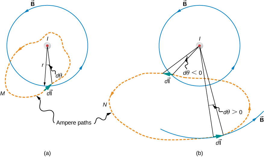
Figure 12.14 shows an arbitrary plane perpendicular to an infinite, straight wire whose current I is directed out of the page. The magnetic field lines are circles directed counterclockwise and centered on the wire. To begin, let’s consider [latex]\oint \stackrel{\to }{\textbf{B}}·d\stackrel{\to }{\textbf{l}}[/latex] over the closed paths M and N. Notice that one path (M) encloses the wire, whereas the other (N) does not. Since the field lines are circular, [latex]\stackrel{\to }{\textbf{B}}·d\stackrel{\to }{\textbf{l}}[/latex] is the product of B and the projection of dl onto the circle passing through [latex]d\stackrel{\to }{\textbf{l}}.[/latex] If the radius of this particular circle is r, the projection is [latex]rd\theta ,[/latex] and
With [latex]\stackrel{\to }{\textbf{B}}[/latex] given by Equation 12.9,
For path M, which circulates around the wire, [latex]{\oint }_{M}d\theta =2\pi[/latex] and
Path N, on the other hand, circulates through both positive (counterclockwise) and negative (clockwise) [latex]d\theta[/latex] (see Figure 12.14), and since it is closed, [latex]{\oint }_{N}d\theta =0.[/latex] Thus for path N,
The extension of this result to the general case is Ampère’s law.
Ampère’s law
Over an arbitrary closed path,
where I is the total current passing through any open surface S whose perimeter is the path of integration. Only currents inside the path of integration need be considered.
To determine whether a specific current I is positive or negative, curl the fingers of your right hand in the direction of the path of integration, as shown in Figure 12.14. If I passes through S in the same direction as your extended thumb, I is positive; if I passes through S in the direction opposite to your extended thumb, it is negative.
Problem-Solving Strategy: Ampère’s Law
To calculate the magnetic field created from current in wire(s), use the following steps:
- Identify the symmetry of the current in the wire(s). If there is no symmetry, use the Biot-Savart law to determine the magnetic field.
- Determine the direction of the magnetic field created by the wire(s) by right-hand rule 2.
- Chose a path loop where the magnetic field is either constant or zero.
- Calculate the current inside the loop.
- Calculate the line integral [latex]\oint \stackrel{\to }{\textbf{B}}·d\stackrel{\to }{\textbf{l}}[/latex] around the closed loop.
- Equate [latex]\oint \stackrel{\to }{\textbf{B}}·d\stackrel{\to }{\textbf{l}}[/latex] with [latex]{\mu }_{0}{I}_{\text{enc}}[/latex] and solve for [latex]\stackrel{\to }{\textbf{B}}.[/latex]
Example
Using Ampère’s Law to Calculate the Magnetic Field Due to a Wire
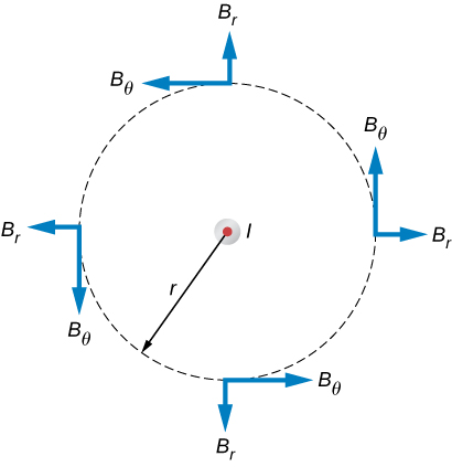
Use Ampère’s law to calculate the magnetic field due to a steady current I in an infinitely long, thin, straight wire as shown in Figure 12.15.
Strategy
Consider an arbitrary plane perpendicular to the wire, with the current directed out of the page. The possible magnetic field components in this plane, [latex]{B}_{r}[/latex] and [latex]{B}_{\theta },[/latex] are shown at arbitrary points on a circle of radius r centered on the wire. Since the field is cylindrically symmetric, neither [latex]{B}_{r}[/latex] nor [latex]{B}_{\theta }[/latex] varies with the position on this circle. Also from symmetry, the radial lines, if they exist, must be directed either all inward or all outward from the wire. This means, however, that there must be a net magnetic flux across an arbitrary cylinder concentric with the wire. The radial component of the magnetic field must be zero because [latex]{\stackrel{\to }{\textbf{B}}}_{r}\cdot d\stackrel{\to }{\textbf{l}}=0.[/latex] Therefore, we can apply Ampère’s law to the circular path as shown.
Solution
Show Answer
Over this path [latex]\stackrel{\to }{\textbf{B}}[/latex] is constant and parallel to [latex]d\stackrel{\to }{\textbf{l}},[/latex] so
Thus Ampère’s law reduces to
Finally, since [latex]{B}_{\theta }[/latex] is the only component of [latex]\stackrel{\to }{\textbf{B}},[/latex] we can drop the subscript and write
This agrees with the Biot-Savart calculation above.
Significance
Ampère’s law works well if you have a path to integrate over which [latex]\stackrel{\to }{\textbf{B}}·d\stackrel{\to }{\textbf{l}}[/latex] has results that are easy to simplify. For the infinite wire, this works easily with a path that is circular around the wire so that the magnetic field factors out of the integration. If the path dependence looks complicated, you can always go back to the Biot-Savart law and use that to find the magnetic field.
Example
Calculating the Magnetic Field of a Thick Wire with Ampère’s Law
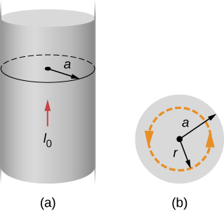
The radius of the long, straight wire of Figure 12.16 is a, and the wire carries a current [latex]{I}_{0}[/latex] that is distributed uniformly over its cross-section. Find the magnetic field both inside and outside the wire.
Strategy
This problem has the same geometry as Example 12.6, but the enclosed current changes as we move the integration path from outside the wire to inside the wire, where it doesn’t capture the entire current enclosed (see Figure 12.16).
Solution
Show Answer
For any circular path of radius r that is centered on the wire,
From Ampère’s law, this equals the total current passing through any surface bounded by the path of integration.
Consider first a circular path that is inside the wire [latex]\left(r\le a\right)[/latex] such as that shown in part (a) of Figure 12.16. We need the current I passing through the area enclosed by the path. It’s equal to the current density J times the area enclosed. Since the current is uniform, the current density inside the path equals the current density in the whole wire, which is [latex]{I}_{0}/\pi {a}^{2}.[/latex] Therefore the current I passing through the area enclosed by the path is
We can consider this ratio because the current density J is constant over the area of the wire. Therefore, the current density of a part of the wire is equal to the current density in the whole area. Using Ampère’s law, we obtain
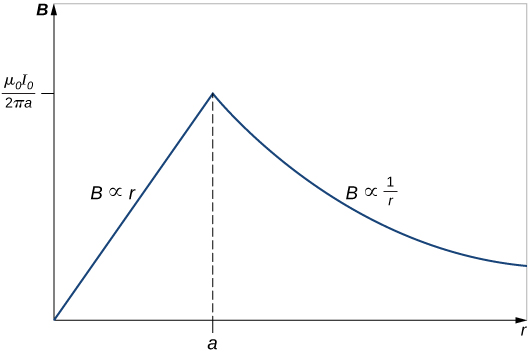
and the magnetic field inside the wire is
Outside the wire, the situation is identical to that of the infinite thin wire of the previous example; that is,
The variation of B with r is shown in Figure 12.17.

Significance
The results show that as the radial distance increases inside the thick wire, the magnetic field increases from zero to a familiar value of the magnetic field of a thin wire. Outside the wire, the field drops off regardless of whether it was a thick or thin wire.
This result is similar to how Gauss’s law for electrical charges behaves inside a uniform charge distribution, except that Gauss’s law for electrical charges has a uniform volume distribution of charge, whereas Ampère’s law here has a uniform area of current distribution. Also, the drop-off outside the thick wire is similar to how an electric field drops off outside of a linear charge distribution, since the two cases have the same geometry and neither case depends on the configuration of charges or currents once the loop is outside the distribution.
Example
Using Ampère’s Law with Arbitrary Paths
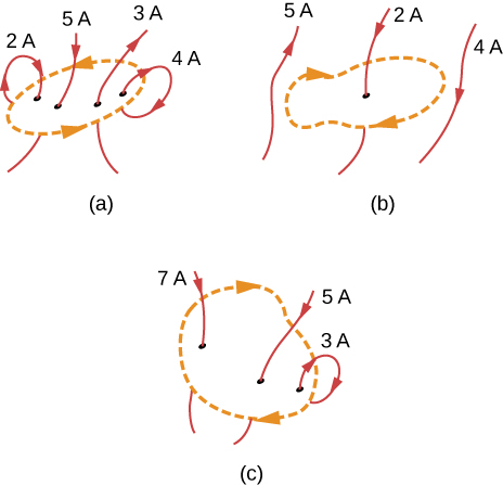
Use Ampère’s law to evaluate [latex]\oint \stackrel{\to }{\textbf{B}}·d\stackrel{\to }{\textbf{l}}[/latex] for the current configurations and paths in Figure 12.18.
Strategy
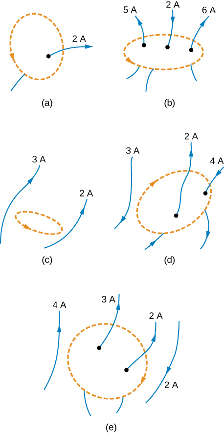
Ampère’s law states that [latex]\oint \stackrel{\to }{\textbf{B}}·d\stackrel{\to }{\textbf{l}}={\mu }_{0}I[/latex] where I is the total current passing through the enclosed loop. The quickest way to evaluate the integral is to calculate [latex]{\mu }_{0}I[/latex] by finding the net current through the loop. Positive currents flow with your right-hand thumb if your fingers wrap around in the direction of the loop. This will tell us the sign of the answer.
Solution
Show Answer
(a) The current going downward through the loop equals the current going out of the loop, so the net current is zero. Thus, [latex]\oint \stackrel{\to }{\textbf{B}}·d\stackrel{\to }{\textbf{l}}=0.[/latex]
(b) The only current to consider in this problem is 2A because it is the only current inside the loop. The right-hand rule shows us the current going downward through the loop is in the positive direction. Therefore, the answer is [latex]\oint \stackrel{\to }{\textbf{B}}·d\stackrel{\to }{\textbf{l}}={\mu }_{0}\left(2\phantom{\rule{0.2em}{0ex}}\text{A}\right)=2.51\phantom{\rule{0.2em}{0ex}}×\phantom{\rule{0.2em}{0ex}}{10}^{\text{−6}}\text{T}\cdot \text{m/A}.[/latex]
(c) The right-hand rule shows us the current going downward through the loop is in the positive direction. There are [latex]\text{7A}+\text{5A}=\text{12A}[/latex] of current going downward and –3 A going upward. Therefore, the total current is 9 A and [latex]\oint \stackrel{\to }{\textbf{B}}·d\stackrel{\to }{\textbf{l}}={\mu }_{0}\left(9\phantom{\rule{0.2em}{0ex}}\text{A}\right)=5.65\phantom{\rule{0.2em}{0ex}}×\phantom{\rule{0.2em}{0ex}}{10}^{\text{−6}}\text{T}\cdot \text{m/A}.[/latex]
Significance
If the currents all wrapped around so that the same current went into the loop and out of the loop, the net current would be zero and no magnetic field would be present. This is why wires are very close to each other in an electrical cord. The currents flowing toward a device and away from a device in a wire equal zero total current flow through an Ampère loop around these wires. Therefore, no stray magnetic fields can be present from cords carrying current.
Check Your Understanding
Consider using Ampère’s law to calculate the magnetic fields of a finite straight wire and of a circular loop of wire. Why is it not useful for these calculations?
Show Solution
In these cases the integrals around the Ampèrian loop are very difficult because there is no symmetry, so this method would not be useful.
Summary
- The magnetic field created by current following any path is the sum (or integral) of the fields due to segments along the path (magnitude and direction as for a straight wire), resulting in a general relationship between current and field known as Ampère’s law.
- Ampère’s law can be used to determine the magnetic field from a thin wire or thick wire by a geometrically convenient path of integration. The results are consistent with the Biot-Savart law.
Conceptual Questions
Is Ampère’s law valid for all closed paths? Why isn’t it normally useful for calculating a magnetic field?
Show Solution
Ampère’s law is valid for all closed paths, but it is not useful for calculating fields when the magnetic field produced lacks symmetry that can be exploited by a suitable choice of path.
Problems
A current I flows around the rectangular loop shown in the accompanying figure. Evaluate [latex]\oint \stackrel{\to }{\textbf{B}}·d\stackrel{\to }{\textbf{l}}[/latex] for the paths A, B, C, and D.
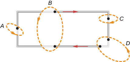
Show Solution
a. [latex]{\mu }_{0}I;[/latex] b. 0; c. [latex]{\mu }_{0}I;[/latex] d. 0
Evaluate [latex]\oint \stackrel{\to }{\textbf{B}}·d\stackrel{\to }{\textbf{l}}[/latex] for each of the cases shown in the accompanying figure.
The coil whose lengthwise cross section is shown in the accompanying figure carries a current I and has N evenly spaced turns distributed along the length l. Evaluate [latex]\oint \stackrel{\to }{\textbf{B}}·d\stackrel{\to }{\textbf{l}}[/latex] for the paths indicated.
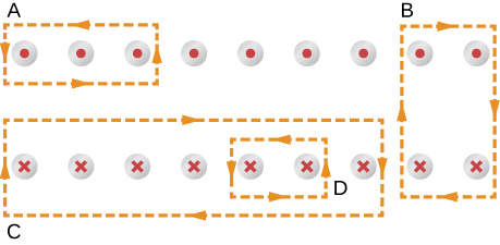
Show Solution
a. [latex]3{\mu }_{0}I;[/latex] b. 0; c. [latex]7{\mu }_{0}I;[/latex] d. [latex]\text{−2}{\mu }_{0}I[/latex]
A superconducting wire of diameter 0.25 cm carries a current of 1000 A. What is the magnetic field just outside the wire?
A long, straight wire of radius R carries a current I that is distributed uniformly over the cross-section of the wire. At what distance from the axis of the wire is the magnitude of the magnetic field a maximum?
Show Solution
at the radius R
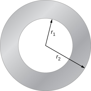
The accompanying figure shows a cross-section of a long, hollow, cylindrical conductor of inner radius [latex]{r}_{1}=\text{3.0 cm}[/latex] and outer radius [latex]{r}_{2}=\text{5.0 cm}.[/latex] A 50-A current distributed uniformly over the cross-section flows into the page. Calculate the magnetic field at [latex]r=\text{2.0 cm},\phantom{\rule{0.2em}{0ex}}r=4.0\phantom{\rule{0.2em}{0ex}}\text{cm},\phantom{\rule{0.2em}{0ex}}\text{and}\phantom{\rule{0.2em}{0ex}}r=\text{6.0 cm}.[/latex]
A long, solid, cylindrical conductor of radius 3.0 cm carries a current of 50 A distributed uniformly over its cross-section. Plot the magnetic field as a function of the radial distance r from the center of the conductor.
Show Solution
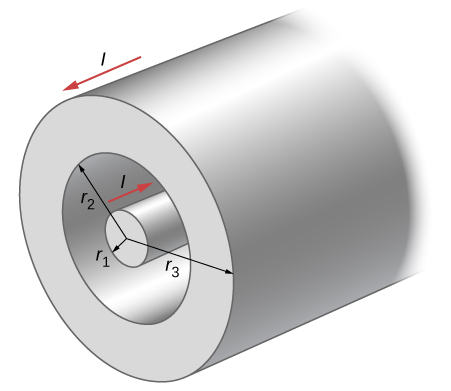
A portion of a long, cylindrical coaxial cable is shown in the accompanying figure. A current I flows down the center conductor, and this current is returned in the outer conductor. Determine the magnetic field in the regions (a) [latex]r\le {r}_{1},[/latex] (b) [latex]{r}_{2}\ge r\ge {r}_{1},[/latex] (c) [latex]{r}_{3}\ge r\ge {r}_{2},[/latex] and (d) [latex]r\ge {r}_{3}.[/latex] Assume that the current is distributed uniformly over the cross sections of the two parts of the cable.
Glossary
- Ampère’s law
- physical law that states that the line integral of the magnetic field around an electric current is proportional to the current
Licenses and Attributions
Ampère’s Law. Authored by: OpenStax College. Located at: https://openstax.org/books/university-physics-volume-2/pages/12-5-amperes-law. License: CC BY: Attribution. License Terms: Download for free at https://openstax.org/books/university-physics-volume-2/pages/1-introduction
