
Chapter 7. Electric Potential
7.3 Calculations of Electric Potential
Learning Objectives
By the end of this section, you will be able to:
- Calculate the potential due to a point charge
- Calculate the potential of a system of multiple point charges
- Describe an electric dipole
- Define dipole moment
- Calculate the potential of a continuous charge distribution
Point charges, such as electrons, are among the fundamental building blocks of matter. Furthermore, spherical charge distributions (such as charge on a metal sphere) create external electric fields exactly like a point charge. The electric potential due to a point charge is, thus, a case we need to consider.
We can use calculus to find the work needed to move a test charge q from a large distance away to a distance of r from a point charge q. Noting the connection between work and potential [latex]W=\text{−}q\text{Δ}V,[/latex] as in the last section, we can obtain the following result.
Electric Potential V of a Point Charge
The electric potential V of a point charge is given by
where k is a constant equal to [latex]8.99\phantom{\rule{0.2em}{0ex}}×\phantom{\rule{0.2em}{0ex}}{10}^{9}\phantom{\rule{0.2em}{0ex}}\text{N}·{\text{m}}^{2}{\text{/C}}^{2}.[/latex]
The potential at infinity is chosen to be zero. Thus, V for a point charge decreases with distance, whereas [latex]\stackrel{\to }{\textbf{E}}[/latex] for a point charge decreases with distance squared:
Recall that the electric potential V is a scalar and has no direction, whereas the electric field [latex]\stackrel{\to }{\textbf{E}}[/latex] is a vector. To find the voltage due to a combination of point charges, you add the individual voltages as numbers. To find the total electric field, you must add the individual fields as vectors, taking magnitude and direction into account. This is consistent with the fact that V is closely associated with energy, a scalar, whereas [latex]\stackrel{\to }{\textbf{E}}[/latex] is closely associated with force, a vector.
Example
What Voltage Is Produced by a Small Charge on a Metal Sphere?
Charges in static electricity are typically in the nanocoulomb (nC) to microcoulomb [latex]\left(\mu \text{C}\right)[/latex] range. What is the voltage 5.00 cm away from the center of a 1-cm-diameter solid metal sphere that has a –3.00-nC static charge?
Strategy
As we discussed in Electric Charges and Fields, charge on a metal sphere spreads out uniformly and produces a field like that of a point charge located at its center. Thus, we can find the voltage using the equation [latex]V=\frac{kq}{r}.[/latex]
Solution
Show Answer
Entering known values into the expression for the potential of a point charge, we obtain
Significance
The negative value for voltage means a positive charge would be attracted from a larger distance, since the potential is lower (more negative) than at larger distances. Conversely, a negative charge would be repelled, as expected.
Example
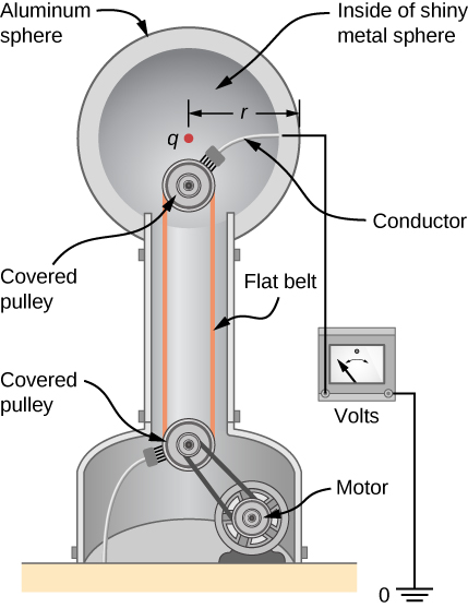
What Is the Excess Charge on a Van de Graaff Generator?
A demonstration Van de Graaff generator has a 25.0-cm-diameter metal sphere that produces a voltage of 100 kV near its surface (Figure 7.18). What excess charge resides on the sphere? (Assume that each numerical value here is shown with three significant figures.)
Strategy
The potential on the surface is the same as that of a point charge at the center of the sphere, 12.5 cm away. (The radius of the sphere is 12.5 cm.) We can thus determine the excess charge using the equation
Solution
Show Answer
Solving for q and entering known values gives
Significance
This is a relatively small charge, but it produces a rather large voltage. We have another indication here that it is difficult to store isolated charges.
Check Your Understanding
What is the potential inside the metal sphere in Example 7.10?
Show Solution
[latex]V=k\frac{q}{r}=\left(8.99\phantom{\rule{0.2em}{0ex}}×\phantom{\rule{0.2em}{0ex}}{10}^{9}\phantom{\rule{0.2em}{0ex}}\text{N}·{\text{m}}^{2}{\text{/C}}^{2}\right)\left(\frac{-3.00\phantom{\rule{0.2em}{0ex}}×\phantom{\rule{0.2em}{0ex}}{10}^{-9}\phantom{\rule{0.2em}{0ex}}\text{C}}{5.00\phantom{\rule{0.2em}{0ex}}×\phantom{\rule{0.2em}{0ex}}{10}^{-3}\phantom{\rule{0.2em}{0ex}}\text{m}}\right)=-5390\phantom{\rule{0.2em}{0ex}}\text{V;}[/latex] recall that the electric field inside a conductor is zero. Hence, any path from a point on the surface to any point in the interior will have an integrand of zero when calculating the change in potential, and thus the potential in the interior of the sphere is identical to that on the surface.
The voltages in both of these examples could be measured with a meter that compares the measured potential with ground potential. Ground potential is often taken to be zero (instead of taking the potential at infinity to be zero). It is the potential difference between two points that is of importance, and very often there is a tacit assumption that some reference point, such as Earth or a very distant point, is at zero potential. As noted earlier, this is analogous to taking sea level as [latex]h=0[/latex] when considering gravitational potential energy [latex]{U}_{g}=mgh[/latex].
Systems of Multiple Point Charges
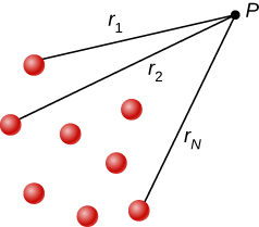
Just as the electric field obeys a superposition principle, so does the electric potential. Consider a system consisting of N charges [latex]{q}_{1},{q}_{2},\text{…},{q}_{N}.[/latex] What is the net electric potential V at a space point P from these charges? Each of these charges is a source charge that produces its own electric potential at point P, independent of whatever other changes may be doing. Let [latex]{V}_{1},{V}_{2},\text{…},{V}_{N}[/latex] be the electric potentials at P produced by the charges [latex]{q}_{1},{q}_{2},\text{…},{q}_{N},[/latex] respectively. Then, the net electric potential [latex]{V}_{P}[/latex] at that point is equal to the sum of these individual electric potentials. You can easily show this by calculating the potential energy of a test charge when you bring the test charge from the reference point at infinity to point P:
Note that electric potential follows the same principle of superposition as electric field and electric potential energy. To show this more explicitly, note that a test charge [latex]{q}_{i}[/latex] at the point P in space has distances of [latex]{r}_{1},{r}_{2},\text{…},{r}_{N}[/latex] from the N charges fixed in space above, as shown in Figure 7.19. Using our formula for the potential of a point charge for each of these (assumed to be point) charges, we find that
Therefore, the electric potential energy of the test charge is
which is the same as the work to bring the test charge into the system, as found in the first section of the chapter.
The Electric Dipole
An electric dipole is a system of two equal but opposite charges a fixed distance apart. This system is used to model many real-world systems, including atomic and molecular interactions. One of these systems is the water molecule, under certain circumstances. These circumstances are met inside a microwave oven, where electric fields with alternating directions make the water molecules change orientation. This vibration is the same as heat at the molecular level.
Example
Electric Potential of a Dipole
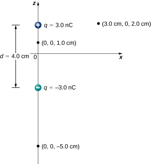
Consider the dipole in Figure 7.20 with the charge magnitude of [latex]q=3.0\phantom{\rule{0.2em}{0ex}}\text{nC}[/latex] and separation distance [latex]d=4.0\phantom{\rule{0.2em}{0ex}}\text{cm}\text{.}[/latex] What is the potential at the following locations in space? (a) (0, 0, 1.0 cm); (b) (0, 0, –5.0 cm); (c) (3.0 cm, 0, 2.0 cm).
Strategy
Apply [latex]{V}_{P}=k\sum _{1}^{N}\frac{{q}_{i}}{{r}_{i}}[/latex] to each of these three points.
Solution
Show Answer
- [latex]{V}_{P}=k\sum _{1}^{N}\frac{{q}_{i}}{{r}_{i}}=\left(9.0\phantom{\rule{0.2em}{0ex}}×\phantom{\rule{0.2em}{0ex}}{10}^{9}\phantom{\rule{0.2em}{0ex}}\text{N}·{\text{m}}^{2}\text{/}{\text{C}}^{2}\right)\left(\frac{3.0\phantom{\rule{0.2em}{0ex}}\text{nC}}{0.010\phantom{\rule{0.2em}{0ex}}\text{m}}-\frac{3.0\phantom{\rule{0.2em}{0ex}}\text{nC}}{0.030\phantom{\rule{0.2em}{0ex}}\text{m}}\right)=1.8\phantom{\rule{0.2em}{0ex}}×\phantom{\rule{0.2em}{0ex}}{10}^{3}\phantom{\rule{0.2em}{0ex}}\text{V}[/latex]
- [latex]{V}_{P}=k\sum _{1}^{N}\frac{{q}_{i}}{{r}_{i}}=\left(9.0\phantom{\rule{0.2em}{0ex}}×\phantom{\rule{0.2em}{0ex}}{10}^{9}\phantom{\rule{0.2em}{0ex}}\text{N}·{\text{m}}^{2}\text{/}{\text{C}}^{2}\right)\left(\frac{3.0\phantom{\rule{0.2em}{0ex}}\text{nC}}{0.070\phantom{\rule{0.2em}{0ex}}\text{m}}-\frac{3.0\phantom{\rule{0.2em}{0ex}}\text{nC}}{0.030\phantom{\rule{0.2em}{0ex}}\text{m}}\right)=-5.1\phantom{\rule{0.2em}{0ex}}×\phantom{\rule{0.2em}{0ex}}{10}^{2}\phantom{\rule{0.2em}{0ex}}\text{V}[/latex]
- [latex]{V}_{P}=k\sum _{1}^{N}\frac{{q}_{i}}{{r}_{i}}=\left(9.0\phantom{\rule{0.2em}{0ex}}×\phantom{\rule{0.2em}{0ex}}{10}^{9}\phantom{\rule{0.2em}{0ex}}\text{N}·{\text{m}}^{2}\text{/}{\text{C}}^{2}\right)\left(\frac{3.0\phantom{\rule{0.2em}{0ex}}\text{nC}}{0.030\phantom{\rule{0.2em}{0ex}}\text{m}}-\frac{3.0\phantom{\rule{0.2em}{0ex}}\text{nC}}{0.050\phantom{\rule{0.2em}{0ex}}\text{m}}\right)=3.6\phantom{\rule{0.2em}{0ex}}×\phantom{\rule{0.2em}{0ex}}{10}^{2}\phantom{\rule{0.2em}{0ex}}\text{V}[/latex]
Significance
Note that evaluating potential is significantly simpler than electric field, due to potential being a scalar instead of a vector.
Check Your Understanding
What is the potential on the x-axis? The z-axis?
Show Solution
The x-axis the potential is zero, due to the equal and opposite charges the same distance from it. On the z-axis, we may superimpose the two potentials; we will find that for [latex]z\phantom{\rule{0.2em}{0ex}}>>\phantom{\rule{0.2em}{0ex}}d[/latex], again the potential goes to zero due to cancellation.
Now let us consider the special case when the distance of the point P from the dipole is much greater than the distance between the charges in the dipole, [latex]r\gg d;[/latex] for example, when we are interested in the electric potential due to a polarized molecule such as a water molecule. This is not so far (infinity) that we can simply treat the potential as zero, but the distance is great enough that we can simplify our calculations relative to the previous example.
We start by noting that in Figure 7.21 the potential is given by
where
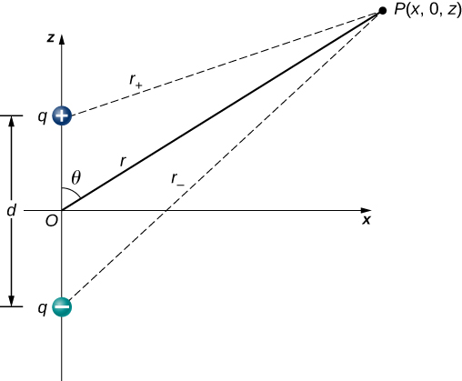
This is still the exact formula. To take advantage of the fact that [latex]r\gg d,[/latex] we rewrite the radii in terms of polar coordinates, with [latex]x=r\phantom{\rule{0.2em}{0ex}}\text{sin}\phantom{\rule{0.2em}{0ex}}\theta[/latex] and [latex]z=r\phantom{\rule{0.2em}{0ex}}\text{cos}\phantom{\rule{0.2em}{0ex}}\theta[/latex]. This gives us
We can simplify this expression by pulling r out of the root,
and then multiplying out the parentheses
The last term in the root is small enough to be negligible (remember [latex]r\gg d,[/latex] and hence [latex]{\left(d\text{/}r\right)}^{2}[/latex] is extremely small, effectively zero to the level we will probably be measuring), leaving us with
Using the binomial approximation (a standard result from the mathematics of series, when [latex]\alpha[/latex] is small)
and substituting this into our formula for [latex]{V}_{P}[/latex] , we get
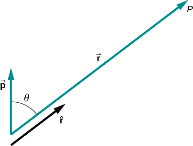
This may be written more conveniently if we define a new quantity, the electric dipole moment,
where these vectors point from the negative to the positive charge. Note that this has magnitude qd. This quantity allows us to write the potential at point P due to a dipole at the origin as
A diagram of the application of this formula is shown in Figure 7.22.
There are also higher-order moments, for quadrupoles, octupoles, and so on. You will see these in future classes.
Potential of Continuous Charge Distributions
We have been working with point charges a great deal, but what about continuous charge distributions? Recall from Equation 7.9 that
We may treat a continuous charge distribution as a collection of infinitesimally separated individual points. This yields the integral
for the potential at a point P. Note that r is the distance from each individual point in the charge distribution to the point P. As we saw in Electric Charges and Fields, the infinitesimal charges are given by
where [latex]\lambda[/latex] is linear charge density, [latex]\sigma[/latex] is the charge per unit area, and [latex]\rho[/latex] is the charge per unit volume.
Example
Potential of a Line of Charge
Find the electric potential of a uniformly charged, nonconducting wire with linear density [latex]\lambda[/latex] (coulomb/meter) and length L at a point that lies on a line that divides the wire into two equal parts.
Strategy
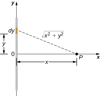
To set up the problem, we choose Cartesian coordinates in such a way as to exploit the symmetry in the problem as much as possible. We place the origin at the center of the wire and orient the y-axis along the wire so that the ends of the wire are at [latex]y=±L\text{/}2[/latex]. The field point P is in the xy-plane and since the choice of axes is up to us, we choose the x-axis to pass through the field point P, as shown in Figure 7.23.
Solution
Show Answer
Consider a small element of the charge distribution between y and [latex]y+dy[/latex]. The charge in this cell is [latex]dq=\lambda \phantom{\rule{0.2em}{0ex}}dy[/latex] and the distance from the cell to the field point P is [latex]\sqrt{{x}^{2}+{y}^{2}}.[/latex] Therefore, the potential becomes
Significance
Note that this was simpler than the equivalent problem for electric field, due to the use of scalar quantities. Recall that we expect the zero level of the potential to be at infinity, when we have a finite charge. To examine this, we take the limit of the above potential as x approaches infinity; in this case, the terms inside the natural log approach one, and hence the potential approaches zero in this limit. Note that we could have done this problem equivalently in cylindrical coordinates; the only effect would be to substitute r for x and z for y.
Example
Potential Due to a Ring of Charge
A ring has a uniform charge density [latex]\lambda[/latex], with units of coulomb per unit meter of arc. Find the electric potential at a point on the axis passing through the center of the ring.
Strategy
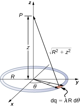
We use the same procedure as for the charged wire. The difference here is that the charge is distributed on a circle. We divide the circle into infinitesimal elements shaped as arcs on the circle and use cylindrical coordinates shown in Figure 7.24.
Solution
Show Answer
A general element of the arc between [latex]\theta[/latex] and [latex]\theta +d\theta[/latex] is of length [latex]Rd\theta[/latex] and therefore contains a charge equal to [latex]\lambda Rd\theta .[/latex] The element is at a distance of [latex]\sqrt{{z}^{2}+{R}^{2}}[/latex] from P, and therefore the potential is
Significance
This result is expected because every element of the ring is at the same distance from point P. The net potential at P is that of the total charge placed at the common distance, [latex]\sqrt{{z}^{2}+{R}^{2}}[/latex].
Example
Potential Due to a Uniform Disk of Charge
A disk of radius R has a uniform charge density [latex]\sigma[/latex], with units of coulomb meter squared. Find the electric potential at any point on the axis passing through the center of the disk.
Strategy
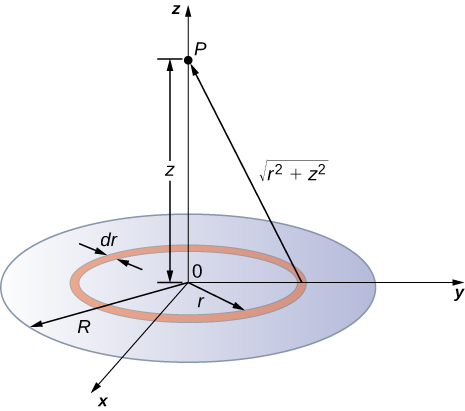
We divide the disk into ring-shaped cells, and make use of the result for a ring worked out in the previous example, then integrate over r in addition to [latex]\theta[/latex]. This is shown in Figure 7.25.
Solution
Show Answer
An infinitesimal width cell between cylindrical coordinates r and [latex]r+dr[/latex] shown in Figure 7.25 will be a ring of charges whose electric potential [latex]d{V}_{P}[/latex] at the field point has the following expression
where
The superposition of potential of all the infinitesimal rings that make up the disk gives the net potential at point P. This is accomplished by integrating from [latex]r=0[/latex] to [latex]r=R[/latex]:
Significance
The basic procedure for a disk is to first integrate around [latex]\theta[/latex] and then over r. This has been demonstrated for uniform (constant) charge density. Often, the charge density will vary with r, and then the last integral will give different results.
Example
Potential Due to an Infinite Charged Wire
Find the electric potential due to an infinitely long uniformly charged wire.
Strategy
Since we have already worked out the potential of a finite wire of length L in Example 7.7, we might wonder if taking [latex]L\to \infty[/latex] in our previous result will work:
However, this limit does not exist because the argument of the logarithm becomes [2/0] as [latex]L\to \infty[/latex], so this way of finding V of an infinite wire does not work. The reason for this problem may be traced to the fact that the charges are not localized in some space but continue to infinity in the direction of the wire. Hence, our (unspoken) assumption that zero potential must be an infinite distance from the wire is no longer valid.
To avoid this difficulty in calculating limits, let us use the definition of potential by integrating over the electric field from the previous section, and the value of the electric field from this charge configuration from the previous chapter.
Solution
Show Answer
We use the integral
where R is a finite distance from the line of charge, as shown in Figure 7.26.
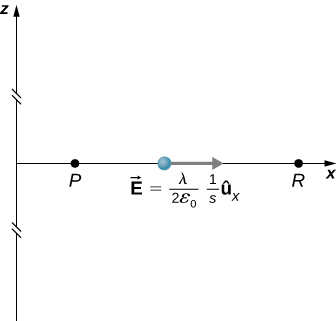
With this setup, we use [latex]{\stackrel{\to }{\textbf{E}}}_{P}=2k\lambda \frac{1}{s}\hat{\textbf{s}}[/latex] and [latex]d\stackrel{\to }{\textbf{l}}=d\stackrel{\to }{\textbf{s}}[/latex] to obtain
Now, if we define the reference potential [latex]{V}_{R}=0[/latex] at [latex]{s}_{R}=1\phantom{\rule{0.2em}{0ex}}\text{m,}[/latex] this simplifies to
Note that this form of the potential is quite usable; it is 0 at 1 m and is undefined at infinity, which is why we could not use the latter as a reference.
Significance
Although calculating potential directly can be quite convenient, we just found a system for which this strategy does not work well. In such cases, going back to the definition of potential in terms of the electric field may offer a way forward.
Check Your Understanding
What is the potential on the axis of a nonuniform ring of charge, where the charge density is [latex]\lambda \left(\theta \right)=\lambda \phantom{\rule{0.2em}{0ex}}\text{cos}\phantom{\rule{0.2em}{0ex}}\theta[/latex] ?
Show Solution
It will be zero, as at all points on the axis, there are equal and opposite charges equidistant from the point of interest. Note that this distribution will, in fact, have a dipole moment.
Summary
- Electric potential is a scalar whereas electric field is a vector.
- Addition of voltages as numbers gives the voltage due to a combination of point charges, allowing us to use the principle of superposition: [latex]{V}_{P}=k\sum _{1}^{N}\frac{{q}_{i}}{{r}_{i}}[/latex].
- An electric dipole consists of two equal and opposite charges a fixed distance apart, with a dipole moment [latex]\stackrel{\to }{\textbf{p}}=q\stackrel{\to }{\textbf{d}}[/latex].
- Continuous charge distributions may be calculated with [latex]{V}_{P}=k\int \frac{dq}{r}[/latex].
Conceptual Questions
Compare the electric dipole moments of charges [latex]±Q[/latex] separated by a distance d and charges [latex]±Q\text{/}2[/latex] separated by a distance d/2.
Show Solution
The second has 1/4 the dipole moment of the first.
Would Gauss’s law be helpful for determining the electric field of a dipole? Why?
In what region of space is the potential due to a uniformly charged sphere the same as that of a point charge? In what region does it differ from that of a point charge?
Show Solution
The region outside of the sphere will have a potential indistinguishable from a point charge; the interior of the sphere will have a different potential.
Can the potential of a nonuniformly charged sphere be the same as that of a point charge? Explain.
Problems
A 0.500-cm-diameter plastic sphere, used in a static electricity demonstration, has a uniformly distributed 40.0-pC charge on its surface. What is the potential near its surface?
Show Solution
[latex]V=144\phantom{\rule{0.2em}{0ex}}\text{V}[/latex]
How far from a [latex]1.00\text{-}\mu \text{C}[/latex] point charge is the potential 100 V? At what distance is it [latex]2.00\phantom{\rule{0.2em}{0ex}}×\phantom{\rule{0.2em}{0ex}}{10}^{2}\phantom{\rule{0.2em}{0ex}}\text{V?}[/latex]
If the potential due to a point charge is [latex]5.00\phantom{\rule{0.2em}{0ex}}×\phantom{\rule{0.2em}{0ex}}{10}^{2}\phantom{\rule{0.2em}{0ex}}\text{V}[/latex] at a distance of 15.0 m, what are the sign and magnitude of the charge?
Show Solution
[latex]V=\frac{kQ}{r}\to Q=8.33\phantom{\rule{0.2em}{0ex}}×\phantom{\rule{0.2em}{0ex}}{10}^{-7}\phantom{\rule{0.2em}{0ex}}\text{C}[/latex];
The charge is positive because the potential is positive.
In nuclear fission, a nucleus splits roughly in half. (a) What is the potential [latex]2.00\phantom{\rule{0.2em}{0ex}}×\phantom{\rule{0.2em}{0ex}}{10}^{-14}\phantom{\rule{0.2em}{0ex}}\text{m}[/latex] from a fragment that has 46 protons in it? (b) What is the potential energy in MeV of a similarly charged fragment at this distance?
A research Van de Graaff generator has a 2.00-m-diameter metal sphere with a charge of 5.00 mC on it. Assume the potential energy is zero at a reference point infinitely far away from the Van de Graaff. (a) What is the potential near its surface? (b) At what distance from its center is the potential 1.00 MV? (c) An oxygen atom with three missing electrons is released near the Van de Graaff generator. What is its energy in MeV when the atom is at the distance found in part b?
Show Solution
a. [latex]V=45.0\phantom{\rule{0.2em}{0ex}}\text{MV}[/latex];
b. [latex]V=\frac{kQ}{r}\to r=45.0\phantom{\rule{0.2em}{0ex}}\text{m}[/latex];
c. [latex]\text{Δ}U=132\phantom{\rule{0.2em}{0ex}}\text{MeV}[/latex]
An electrostatic paint sprayer has a 0.200-m-diameter metal sphere at a potential of 25.0 kV that repels paint droplets onto a grounded object.
(a) What charge is on the sphere? (b) What charge must a 0.100-mg drop of paint have to arrive at the object with a speed of 10.0 m/s?
(a) What is the potential between two points situated 10 cm and 20 cm from a [latex]3.0\text{-}\mu \text{C}[/latex] point charge? (b) To what location should the point at 20 cm be moved to increase this potential difference by a factor of two?
Show Solution
[latex]V=kQ/r[/latex]; a. Relative to origin, find the potential at each point and then calculate the difference.
[latex]\text{Δ}V=135\phantom{\rule{0.2em}{0ex}}×\phantom{\rule{0.2em}{0ex}}{10}^{3}\phantom{\rule{0.2em}{0ex}}\text{V}[/latex];
b. To double the potential difference, move the point from 20 cm to infinity; the potential at 20 cm is halfway between zero and that at 10 cm.
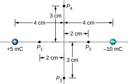
Find the potential at points [latex]{P}_{1},{P}_{2},{P}_{3},\phantom{\rule{0.2em}{0ex}}\text{and}\phantom{\rule{0.2em}{0ex}}{P}_{4}[/latex] in the diagram due to the two given charges.
Two charges [latex]–2.0\phantom{\rule{0.2em}{0ex}}µ\text{C}\phantom{\rule{0.2em}{0ex}}\text{and}\phantom{\rule{0.2em}{0ex}}\text{+}2.0\phantom{\rule{0.2em}{0ex}}µ\text{C}[/latex] are separated by 4.0 cm on the z-axis symmetrically about origin, with the positive one uppermost. Two space points of interest [latex]{P}_{1}\phantom{\rule{0.2em}{0ex}}\text{and}\phantom{\rule{0.2em}{0ex}}{P}_{2}[/latex] are located 3.0 cm and 30 cm from origin at an angle [latex]30\text{°}[/latex] with respect to the z-axis. Evaluate electric potentials at [latex]{P}_{1}\phantom{\rule{0.2em}{0ex}}\text{and}\phantom{\rule{0.2em}{0ex}}{P}_{2}[/latex] in two ways: (a) Using the exact formula for point charges, and (b) using the approximate dipole potential formula.
Show Solution
a. [latex]{V}_{P1}=7.4\phantom{\rule{0.2em}{0ex}}×\phantom{\rule{0.2em}{0ex}}{10}^{5}\phantom{\rule{0.2em}{0ex}}\text{V}[/latex]
and [latex]{V}_{P2}=6.9\phantom{\rule{0.2em}{0ex}}×\phantom{\rule{0.2em}{0ex}}{10}^{3}\phantom{\rule{0.2em}{0ex}}\text{V}[/latex];
b. [latex]{V}_{P1}=6.9\phantom{\rule{0.2em}{0ex}}×\phantom{\rule{0.2em}{0ex}}{10}^{5}\phantom{\rule{0.2em}{0ex}}\text{V}[/latex] and [latex]{V}_{P2}=6.9\phantom{\rule{0.2em}{0ex}}×\phantom{\rule{0.2em}{0ex}}{10}^{3}\phantom{\rule{0.2em}{0ex}}\text{V}[/latex]
(a) Plot the potential of a uniformly charged 1-m rod with 1 C/m charge as a function of the perpendicular distance from the center. Draw your graph from [latex]\text{s}=0.1\phantom{\rule{0.2em}{0ex}}\text{m}\phantom{\rule{0.2em}{0ex}}\text{to}\phantom{\rule{0.2em}{0ex}}\text{s}=1.0\phantom{\rule{0.2em}{0ex}}\text{m}[/latex]. (b) On the same graph, plot the potential of a point charge with a 1-C charge at the origin. (c) Which potential is stronger near the rod? (d) What happens to the difference as the distance increases? Interpret your result.
Glossary
- electric dipole
- system of two equal but opposite charges a fixed distance apart
- electric dipole moment
- quantity defined as [latex]\stackrel{\to }{\textbf{p}}=q\stackrel{\to }{\textbf{d}}[/latex] for all dipoles, where the vector points from the negative to positive charge
Licenses and Attributions
Calculations of Electric Potential. Authored by: OpenStax College. Located at: https://openstax.org/books/university-physics-volume-2/pages/7-3-calculations-of-electric-potential. License: CC BY: Attribution. License Terms: Download for free at https://openstax.org/books/university-physics-volume-2/pages/1-introduction
