
Chapter 16. Electromagnetic Waves
16.2 Plane Electromagnetic Waves
Learning Objectives
By the end of this section, you will be able to:
- Describe how Maxwell’s equations predict the relative directions of the electric fields and magnetic fields, and the direction of propagation of plane electromagnetic waves
- Explain how Maxwell’s equations predict that the speed of propagation of electromagnetic waves in free space is exactly the speed of light
- Calculate the relative magnitude of the electric and magnetic fields in an electromagnetic plane wave
- Describe how electromagnetic waves are produced and detected
Mechanical waves travel through a medium such as a string, water, or air. Perhaps the most significant prediction of Maxwell’s equations is the existence of combined electric and magnetic (or electromagnetic) fields that propagate through space as electromagnetic waves. Because Maxwell’s equations hold in free space, the predicted electromagnetic waves, unlike mechanical waves, do not require a medium for their propagation.
A general treatment of the physics of electromagnetic waves is beyond the scope of this textbook. We can, however, investigate the special case of an electromagnetic wave that propagates through free space along the x-axis of a given coordinate system.
Electromagnetic Waves in One Direction
An electromagnetic wave consists of an electric field, defined as usual in terms of the force per charge on a stationary charge, and a magnetic field, defined in terms of the force per charge on a moving charge. The electromagnetic field is assumed to be a function of only the x-coordinate and time. The y-component of the electric field is then written as [latex]{E}_{y}\left(x,t\right),[/latex] the z-component of the magnetic field as [latex]{B}_{z}\left(x,t\right)[/latex], etc. Because we are assuming free space, there are no free charges or currents, so we can set [latex]{Q}_{\text{in}}=0[/latex] and [latex]I=0[/latex] in Maxwell’s equations.
The transverse nature of electromagnetic waves
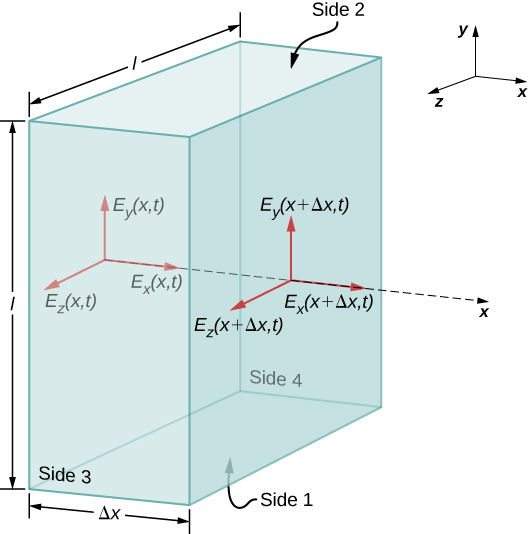
We examine first what Gauss’s law for electric fields implies about the relative directions of the electric field and the propagation direction in an electromagnetic wave. Assume the Gaussian surface to be the surface of a rectangular box whose cross-section is a square of side l and whose third side has length [latex]\text{Δ}x[/latex], as shown in Figure 16.6. Because the electric field is a function only of x and t, the y-component of the electric field is the same on both the top (labeled Side 2) and bottom (labeled Side 1) of the box, so that these two contributions to the flux cancel. The corresponding argument also holds for the net flux from the z-component of the electric field through Sides 3 and 4. Any net flux through the surface therefore comes entirely from the x-component of the electric field. Because the electric field has no y- or z-dependence, [latex]{E}_{x}\left(x,t\right)[/latex] is constant over the face of the box with area A and has a possibly different value [latex]{E}_{x}\left(x+\text{Δ}x,t\right)[/latex] that is constant over the opposite face of the box. Applying Gauss’s law gives
where [latex]A=l\phantom{\rule{0.2em}{0ex}}×\phantom{\rule{0.2em}{0ex}}l[/latex] is the area of the front and back faces of the rectangular surface. But the charge enclosed is [latex]{Q}_{\text{in}}=0[/latex], so this component’s net flux is also zero, and Equation 16.13 implies [latex]{E}_{x}\left(x,t\right)={E}_{x}\left(x+\text{Δ}x,t\right)[/latex] for any [latex]\text{Δ}x[/latex]. Therefore, if there is an x-component of the electric field, it cannot vary with x. A uniform field of that kind would merely be superposed artificially on the traveling wave, for example, by having a pair of parallel-charged plates. Such a component [latex]{E}_{x}\left(x,t\right)[/latex] would not be part of an electromagnetic wave propagating along the x-axis; so [latex]{E}_{x}\left(x,t\right)=0[/latex] for this wave. Therefore, the only nonzero components of the electric field are [latex]{E}_{y}\left(x,t\right)[/latex] and [latex]{E}_{z}\left(x,t\right),[/latex] perpendicular to the direction of propagation of the wave.
A similar argument holds by substituting E for B and using Gauss’s law for magnetism instead of Gauss’s law for electric fields. This shows that the B field is also perpendicular to the direction of propagation of the wave. The electromagnetic wave is therefore a transverse wave, with its oscillating electric and magnetic fields perpendicular to its direction of propagation.
The speed of propagation of electromagnetic waves
We can next apply Maxwell’s equations to the description given in connection with Figure 16.4 in the previous section to obtain an equation for the E field from the changing B field, and for the B field from a changing E field. We then combine the two equations to show how the changing E and B fields propagate through space at a speed precisely equal to the speed of light.
First, we apply Faraday’s law over Side 3 of the Gaussian surface, using the path shown in Figure 16.7. Because [latex]{E}_{x}\left(x,t\right)=0,[/latex] we have
Assuming [latex]\text{Δ}x[/latex] is small and approximating [latex]{E}_{y}\left(x+\text{Δ}x,t\right)[/latex] by
we obtain
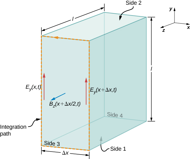
Because [latex]\text{Δ}x[/latex] is small, the magnetic flux through the face can be approximated by its value in the center of the area traversed, namely [latex]{B}_{z}\left(x+\frac{\text{Δ}x}{2},t\right)[/latex]. The flux of the B field through Face 3 is then the B field times the area,
From Faraday’s law,
Therefore, from Equation 16.13 and Equation 16.14,
Canceling [latex]l\text{Δ}x[/latex] and taking the limit as [latex]\text{Δ}x=0[/latex], we are left with
We could have applied Faraday’s law instead to the top surface (numbered 2) in Figure 16.7, to obtain the resulting equation
This is the equation describing the spatially dependent E field produced by the time-dependent B field.
Next we apply the Ampère-Maxwell law (with [latex]I=0[/latex]) over the same two faces (Surface 3 and then Surface 2) of the rectangular box of Figure 16.7. Applying Equation 16.10,
to Surface 3, and then to Surface 2, yields the two equations
These equations describe the spatially dependent B field produced by the time-dependent E field.
We next combine the equations showing the changing B field producing an E field with the equation showing the changing E field producing a B field. Taking the derivative of Equation 16.16 with respect to x and using Equation 16.26 gives
This is the form taken by the general wave equation for our plane wave. Because the equations describe a wave traveling at some as-yet-unspecified speed c, we can assume the field components are each functions of x – ct for the wave traveling in the +x-direction, that is,
It is left as a mathematical exercise to show, using the chain rule for differentiation, that Equation 16.17 and Equation 16.18 imply
The speed of the electromagnetic wave in free space is therefore given in terms of the permeability and the permittivity of free space by
We could just as easily have assumed an electromagnetic wave with field components [latex]{E}_{z}\left(x,t\right)[/latex] and [latex]{B}_{y}\left(x,t\right)[/latex]. The same type of analysis with Equation 16.25 and Equation 16.24 would also show that the speed of an electromagnetic wave is [latex]c=1\text{/}\sqrt{{\epsilon }_{0}{\mu }_{0}}[/latex].
The physics of traveling electromagnetic fields was worked out by Maxwell in 1873. He showed in a more general way than our derivation that electromagnetic waves always travel in free space with a speed given by Equation 16.18. If we evaluate the speed [latex]c=\frac{1}{\sqrt{{\epsilon }_{0}{\mu }_{0}}},[/latex] we find that
which is the speed of light. Imagine the excitement that Maxwell must have felt when he discovered this equation! He had found a fundamental connection between two seemingly unrelated phenomena: electromagnetic fields and light.
Check Your Understanding
The wave equation was obtained by (1) finding the E field produced by the changing B field, (2) finding the B field produced by the changing E field, and combining the two results. Which of Maxwell’s equations was the basis of step (1) and which of step (2)?
Show Solution
(1) Faraday’s law, (2) the Ampère-Maxwell law
How the E and B Fields Are Related
So far, we have seen that the rates of change of different components of the E and B fields are related, that the electromagnetic wave is transverse, and that the wave propagates at speed c. We next show what Maxwell’s equations imply about the ratio of the E and B field magnitudes and the relative directions of the E and B fields.
We now consider solutions to Equation 16.16 in the form of plane waves for the electric field:
We have arbitrarily taken the wave to be traveling in the +x-direction and chosen its phase so that the maximum field strength occurs at the origin at time [latex]t=0[/latex]. We are justified in considering only sines and cosines in this way, and generalizing the results, because Fourier’s theorem implies we can express any wave, including even square step functions, as a superposition of sines and cosines.
At any one specific point in space, the E field oscillates sinusoidally at angular frequency [latex]\omega[/latex] between [latex]+{E}_{0}[/latex] and [latex]\text{−}{E}_{0},[/latex] and similarly, the B field oscillates between [latex]+{B}_{0}[/latex] and [latex]\text{−}{B}_{0}.[/latex] The amplitude of the wave is the maximum value of [latex]{E}_{y}\left(x,t\right).[/latex] The period of oscillation T is the time required for a complete oscillation. The frequency f is the number of complete oscillations per unit of time, and is related to the angular frequency [latex]\omega[/latex] by [latex]\omega =2\pi f[/latex]. The wavelength [latex]\lambda[/latex] is the distance covered by one complete cycle of the wave, and the wavenumber k is the number of wavelengths that fit into a distance of [latex]2\text{π}[/latex] in the units being used. These quantities are related in the same way as for a mechanical wave:
Given that the solution of [latex]{E}_{y}[/latex] has the form shown in Equation 16.20, we need to determine the B field that accompanies it. From Equation 16.24, the magnetic field component [latex]{B}_{z}[/latex] must obey
Because the solution for the B-field pattern of the wave propagates in the +x-direction at the same speed c as the E-field pattern, it must be a function of [latex]k\left(x-ct\right)=kx-\omega t[/latex]. Thus, we conclude from Equation 16.21 that [latex]{B}_{z}[/latex] is
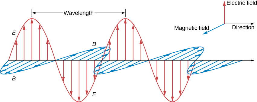
These results may be written as
Therefore, the peaks of the E and B fields coincide, as do the troughs of the wave, and at each point, the E and B fields are in the same ratio equal to the speed of light c. The plane wave has the form shown in Figure 16.8.
Example
Calculating B-Field Strength in an Electromagnetic Wave
What is the maximum strength of the B field in an electromagnetic wave that has a maximum E-field strength of 1000 V/m?
Strategy
To find the B-field strength, we rearrange Equation 16.23 to solve for B, yielding
Solution
Show Answer
We are given E, and c is the speed of light. Entering these into the expression for B yields
Significance
The B-field strength is less than a tenth of Earth’s admittedly weak magnetic field. This means that a relatively strong electric field of 1000 V/m is accompanied by a relatively weak magnetic field.
Changing electric fields create relatively weak magnetic fields. The combined electric and magnetic fields can be detected in electromagnetic waves, however, by taking advantage of the phenomenon of resonance, as Hertz did. A system with the same natural frequency as the electromagnetic wave can be made to oscillate. All radio and TV receivers use this principle to pick up and then amplify weak electromagnetic waves, while rejecting all others not at their resonant frequency.
Check Your Understanding
What conclusions did our analysis of Maxwell’s equations lead to about these properties of a plane electromagnetic wave:
(a) the relative directions of wave propagation, of the E field, and of B field,
(b) the speed of travel of the wave and how the speed depends on frequency, and
(c) the relative magnitudes of the E and B fields.
Show Solution
a. The directions of wave propagation, of the E field, and of B field are all mutually perpendicular. b. The speed of the electromagnetic wave is the speed of light [latex]c=1\text{/}\sqrt{{\epsilon }_{0}{\mu }_{0}}[/latex] independent of frequency. c. The ratio of electric and magnetic field amplitudes is [latex]E\text{/}B=c.[/latex]
Production and Detection of Electromagnetic Waves
A steady electric current produces a magnetic field that is constant in time and which does not propagate as a wave. Accelerating charges, however, produce electromagnetic waves. An electric charge oscillating up and down, or an alternating current or flow of charge in a conductor, emit radiation at the frequencies of their oscillations. The electromagnetic field of a dipole antenna is shown in Figure 16.9. The positive and negative charges on the two conductors are made to reverse at the desired frequency by the output of a transmitter as the power source. The continually changing current accelerates charge in the antenna, and this results in an oscillating electric field a distance away from the antenna. The changing electric fields produce changing magnetic fields that in turn produce changing electric fields, which thereby propagate as electromagnetic waves. The frequency of this radiation is the same as the frequency of the ac source that is accelerating the electrons in the antenna. The two conducting elements of the dipole antenna are commonly straight wires. The total length of the two wires is typically about one-half of the desired wavelength (hence, the alternative name half-wave antenna), because this allows standing waves to be set up and enhances the effectiveness of the radiation.
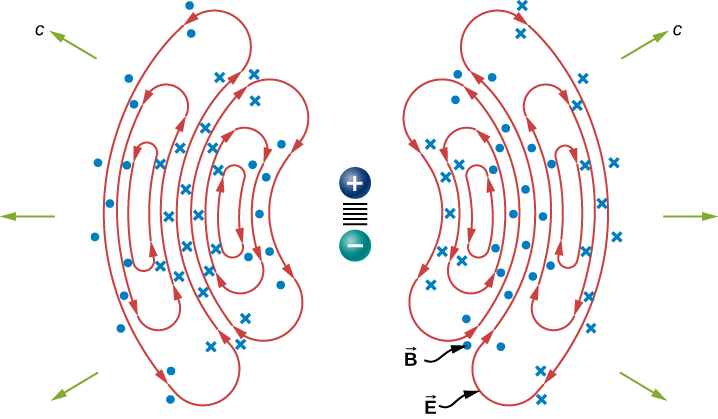
The electric field lines in one plane are shown. The magnetic field is perpendicular to this plane. This radiation field has cylindrical symmetry around the axis of the dipole. Field lines near the dipole are not shown. The pattern is not at all uniform in all directions. The strongest signal is in directions perpendicular to the axis of the antenna, which would be horizontal if the antenna is mounted vertically. There is zero intensity along the axis of the antenna. The fields detected far from the antenna are from the changing electric and magnetic fields inducing each other and traveling as electromagnetic waves. Far from the antenna, the wave fronts, or surfaces of equal phase for the electromagnetic wave, are almost spherical. Even farther from the antenna, the radiation propagates like electromagnetic plane waves.
The electromagnetic waves carry energy away from their source, similar to a sound wave carrying energy away from a standing wave on a guitar string. An antenna for receiving electromagnetic signals works in reverse. Incoming electromagnetic waves induce oscillating currents in the antenna, each at its own frequency. The radio receiver includes a tuner circuit, whose resonant frequency can be adjusted. The tuner responds strongly to the desired frequency but not others, allowing the user to tune to the desired broadcast. Electrical components amplify the signal formed by the moving electrons. The signal is then converted into an audio and/or video format.
Use this simulation to broadcast radio waves. Wiggle the transmitter electron manually or have it oscillate automatically. Display the field as a curve or vectors. The strip chart shows the electron positions at the transmitter and at the receiver.
Summary
- Maxwell’s equations predict that the directions of the electric and magnetic fields of the wave, and the wave’s direction of propagation, are all mutually perpendicular. The electromagnetic wave is a transverse wave.
- The strengths of the electric and magnetic parts of the wave are related by [latex]c=E\text{/}B,[/latex] which implies that the magnetic field B is very weak relative to the electric field E.
- Accelerating charges create electromagnetic waves (for example, an oscillating current in a wire produces electromagnetic waves with the same frequency as the oscillation).
Conceptual Questions
If the electric field of an electromagnetic wave is oscillating along the z-axis and the magnetic field is oscillating along the x-axis, in what possible direction is the wave traveling?
In which situation shown below will the electromagnetic wave be more successful in inducing a current in the wire? Explain.
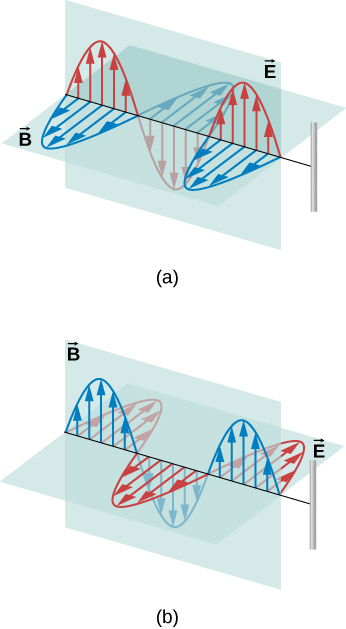
Show Solution
in (a), because the electric field is parallel to the wire, accelerating the electrons
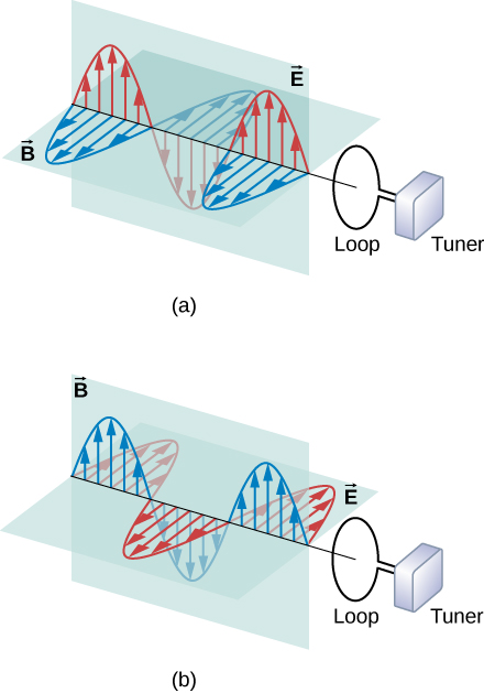
In which situation shown below will the electromagnetic wave be more successful in inducing a current in the loop? Explain.
Under what conditions might wires in a circuit where the current flows in only one direction emit electromagnetic waves?
Show Solution
A steady current in a dc circuit will not produce electromagnetic waves. If the magnitude of the current varies while remaining in the same direction, the wires will emit electromagnetic waves, for example, if the current is turned on or off.
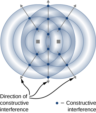
Shown below is the interference pattern of two radio antennas broadcasting the same signal. Explain how this is analogous to the interference pattern for sound produced by two speakers. Could this be used to make a directional antenna system that broadcasts preferentially in certain directions? Explain.
Problems
If the Sun suddenly turned off, we would not know it until its light stopped coming. How long would that be, given that the Sun is [latex]1.496\phantom{\rule{0.2em}{0ex}}×\phantom{\rule{0.2em}{0ex}}{10}^{11}\phantom{\rule{0.2em}{0ex}}\text{m}[/latex] away?
Show Solution
499 s
What is the maximum electric field strength in an electromagnetic wave that has a maximum magnetic field strength of [latex]5.00\phantom{\rule{0.2em}{0ex}}×\phantom{\rule{0.2em}{0ex}}{10}^{-4}\phantom{\rule{0.2em}{0ex}}\text{T}[/latex] (about 10 times Earth’s magnetic field)?
An electromagnetic wave has a frequency of 12 MHz. What is its wavelength in vacuum?
Show Solution
25 m
If electric and magnetic field strengths vary sinusoidally in time at frequency 1.00 GHz, being zero at [latex]t=0[/latex], then [latex]E={E}_{0}\phantom{\rule{0.2em}{0ex}}\text{sin}\phantom{\rule{0.2em}{0ex}}2\pi ft[/latex] and [latex]B={B}_{0}\phantom{\rule{0.2em}{0ex}}\text{sin}\phantom{\rule{0.2em}{0ex}}2\pi ft[/latex]. (a) When are the field strengths next equal to zero? (b) When do they reach their most negative value? (c) How much time is needed for them to complete one cycle?
The electric field of an electromagnetic wave traveling in vacuum is described by the following wave function:
[latex]\stackrel{\to }{\textbf{E}}=\left(5.00\phantom{\rule{0.2em}{0ex}}\text{V/m}\right)\phantom{\rule{0.2em}{0ex}}\text{cos}\phantom{\rule{0.2em}{0ex}}\left[kx-\left(6.00\phantom{\rule{0.2em}{0ex}}×\phantom{\rule{0.2em}{0ex}}{10}^{9}{\phantom{\rule{0.2em}{0ex}}\text{s}}^{-1}\right)t+0.40\right]\hat{\textbf{j}}[/latex]
where k is the wavenumber in rad/m, x is in m, t is in s.
Find the following quantities:
(a) amplitude
(b) frequency
(c) wavelength
(d) the direction of the travel of the wave
(e) the associated magnetic field wave
Show Solution
a. 5.00 V/m; b. [latex]9.55\phantom{\rule{0.2em}{0ex}}×\phantom{\rule{0.2em}{0ex}}{10}^{8}\text{Hz}[/latex]; c. 31.4 cm; d. toward the +x-axis;
e. [latex]B=\left(1.67\phantom{\rule{0.2em}{0ex}}×\phantom{\rule{0.2em}{0ex}}{10}^{-8}\phantom{\rule{0.2em}{0ex}}\text{T}\right)\phantom{\rule{0.2em}{0ex}}\text{cos}\phantom{\rule{0.2em}{0ex}}\left[kx-\left(6\phantom{\rule{0.2em}{0ex}}×\phantom{\rule{0.2em}{0ex}}{10}^{9}{\phantom{\rule{0.2em}{0ex}}\text{s}}^{-1}\right)t+0.40\right]\hat{\textbf{k}}[/latex]
A plane electromagnetic wave of frequency 20 GHz moves in the positive y-axis direction such that its electric field is pointed along the z-axis. The amplitude of the electric field is 10 V/m. The start of time is chosen so that at [latex]t=0[/latex], the electric field has a value 10 V/m at the origin. (a) Write the wave function that will describe the electric field wave. (b) Find the wave function that will describe the associated magnetic field wave.
The following represents an electromagnetic wave traveling in the direction of the positive y-axis: [latex]\begin{array}{c}{E}_{x}=0;{E}_{y}={E}_{0}\phantom{\rule{0.2em}{0ex}}\text{cos}\phantom{\rule{0.2em}{0ex}}\left(kx-\omega t\right);{E}_{z}=0\hfill \\ {B}_{x}=0;{B}_{y}=0;{B}_{z}={B}_{0}\phantom{\rule{0.2em}{0ex}}\text{cos}\phantom{\rule{0.2em}{0ex}}\left(kx-\omega t\right)\hfill \end{array}[/latex].
The wave is passing through a wide tube of circular cross-section of radius R whose axis is along the y-axis. Find the expression for the displacement current through the tube.
Show Solution
[latex]{I}_{\text{d}}=\pi {\epsilon }_{0}\omega {R}^{2}{E}_{0}\phantom{\rule{0.2em}{0ex}}\text{sin}\phantom{\rule{0.2em}{0ex}}\left(kx-\omega t\right)[/latex]
Licenses and Attributions
Plane Electromagnetic Waves. Authored by: OpenStax College. Located at: https://openstax.org/books/university-physics-volume-2/pages/16-2-plane-electromagnetic-waves. License: CC BY: Attribution. License Terms: Download for free at https://openstax.org/books/university-physics-volume-2/pages/1-introduction
