
Chapter 16. Electromagnetic Waves
16.1 Maxwell’s Equations and Electromagnetic Waves
Learning Objectives
By the end of this section, you will be able to:
- Explain Maxwell’s correction of Ampère’s law by including the displacement current
- State and apply Maxwell’s equations in integral form
- Describe how the symmetry between changing electric and changing magnetic fields explains Maxwell’s prediction of electromagnetic waves
- Describe how Hertz confirmed Maxwell’s prediction of electromagnetic waves
James Clerk Maxwell (1831–1879) was one of the major contributors to physics in the nineteenth century (Figure 16.2). Although he died young, he made major contributions to the development of the kinetic theory of gases, to the understanding of color vision, and to the nature of Saturn’s rings. He is probably best known for having combined existing knowledge of the laws of electricity and of magnetism with insights of his own into a complete overarching electromagnetic theory, represented by Maxwell’s equations.
Maxwell’s Correction to the Laws of Electricity and Magnetism
The four basic laws of electricity and magnetism had been discovered experimentally through the work of physicists such as Oersted, Coulomb, Gauss, and Faraday. Maxwell discovered logical inconsistencies in these earlier results and identified the incompleteness of Ampère’s law as their cause.
Recall that according to Ampère’s law, the integral of the magnetic field around a closed loop C is proportional to the current I passing through any surface whose boundary is loop C itself:
There are infinitely many surfaces that can be attached to any loop, and Ampère’s law stated in Equation 16.1 is independent of the choice of surface.
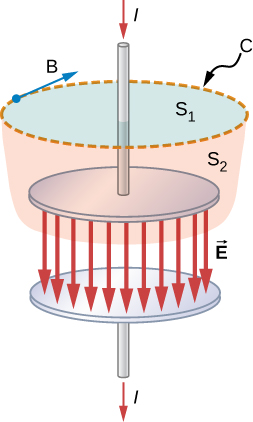
Consider the set-up in Figure 16.3. A source of emf is abruptly connected across a parallel-plate capacitor so that a time-dependent current I develops in the wire. Suppose we apply Ampère’s law to loop C shown at a time before the capacitor is fully charged, so that [latex]I\ne 0[/latex]. Surface [latex]{S}_{1}[/latex] gives a nonzero value for the enclosed current I, whereas surface [latex]{S}_{2}[/latex] gives zero for the enclosed current because no current passes through it:
Clearly, Ampère’s law in its usual form does not work here. This may not be surprising, because Ampère’s law as applied in earlier chapters required a steady current, whereas the current in this experiment is changing with time and is not steady at all.
How can Ampère’s law be modified so that it works in all situations? Maxwell suggested including an additional contribution, called the displacement current [latex]{I}_{\text{d}}[/latex], to the real current I,
where the displacement current is defined to be
Here [latex]{\epsilon }_{0}[/latex] is the permittivity of free space and [latex]{\text{Φ}}_{\text{E}}[/latex] is the electric flux, defined as
The displacement current is analogous to a real current in Ampère’s law, entering into Ampère’s law in the same way. It is produced, however, by a changing electric field. It accounts for a changing electric field producing a magnetic field, just as a real current does, but the displacement current can produce a magnetic field even where no real current is present. When this extra term is included, the modified Ampère’s law equation becomes
and is independent of the surface S through which the current I is measured.
We can now examine this modified version of Ampère’s law to confirm that it holds independent of whether the surface [latex]{S}_{1}[/latex] or the surface [latex]{S}_{2}[/latex] in Figure 16.3 is chosen. The electric field [latex]\stackrel{\to }{\textbf{E}}[/latex] corresponding to the flux [latex]{\text{Φ}}_{E}[/latex] in Equation 16.3 is between the capacitor plates. Therefore, the [latex]\stackrel{\to }{\textbf{E}}[/latex] field and the displacement current through the surface [latex]{S}_{1}[/latex] are both zero, and Equation 16.2 takes the form
We must now show that for surface [latex]{S}_{2},[/latex] through which no actual current flows, the displacement current leads to the same value [latex]{\mu }_{0}I[/latex] for the right side of the Ampère’s law equation. For surface [latex]{S}_{2},[/latex] the equation becomes
Gauss’s law for electric charge requires a closed surface and cannot ordinarily be applied to a surface like [latex]{S}_{1}[/latex] alone or [latex]{S}_{2}[/latex] alone. But the two surfaces [latex]{S}_{1}[/latex] and [latex]{S}_{2}[/latex] form a closed surface in Figure 16.3 and can be used in Gauss’s law. Because the electric field is zero on [latex]{S}_{1}[/latex], the flux contribution through [latex]{S}_{1}[/latex] is zero. This gives us
Therefore, we can replace the integral over [latex]{S}_{2}[/latex] in Equation 16.5 with the closed Gaussian surface [latex]{S}_{1}+{S}_{2}[/latex] and apply Gauss’s law to obtain
Thus, the modified Ampère’s law equation is the same using surface [latex]{S}_{2},[/latex] where the right-hand side results from the displacement current, as it is for the surface [latex]{S}_{1},[/latex] where the contribution comes from the actual flow of electric charge.
Example
Displacement current in a charging capacitor
A parallel-plate capacitor with capacitance C whose plates have area A and separation distance d is connected to a resistor R and a battery of voltage V. The current starts to flow at [latex]t=0[/latex]. (a) Find the displacement current between the capacitor plates at time t. (b) From the properties of the capacitor, find the corresponding real current [latex]I=\frac{dQ}{dt}[/latex], and compare the answer to the expected current in the wires of the corresponding RC circuit.
Strategy
We can use the equations from the analysis of an RC circuit (Alternating-Current Circuits) plus Maxwell’s version of Ampère’s law.
Solution
Show Answer
- The voltage between the plates at time t is given by
[latex]{V}_{C}=\frac{1}{C}Q\left(t\right)={V}_{0}\left(1-{e}^{\text{−}t\text{/}RC}\right).[/latex]
Let the z-axis point from the positive plate to the negative plate. Then the z-component of the electric field between the plates as a function of time t is
[latex]{E}_{z}\left(t\right)=\frac{{V}_{0}}{d}\left(1-{e}^{\text{−}t\text{/}RC}\right).[/latex]
Therefore, the z-component of the displacement current [latex]{I}_{\text{d}}[/latex] between the plates is
[latex]{I}_{\text{d}}\left(t\right)={\epsilon }_{0}A\frac{\partial {E}_{z}\left(t\right)}{\partial t}={\epsilon }_{0}A\frac{{V}_{0}}{d}\phantom{\rule{0.2em}{0ex}}×\phantom{\rule{0.2em}{0ex}}\frac{1}{RC}{e}^{\text{−}t\text{/}RC}=\frac{{V}_{0}}{R}{e}^{\text{−}t\text{/}RC},[/latex]
where we have used [latex]C={\epsilon }_{0}\frac{A}{d}[/latex] for the capacitance. - From the expression for [latex]{V}_{C},[/latex] the charge on the capacitor is
[latex]Q\left(t\right)=C{V}_{C}=C{V}_{0}\left(1-{e}^{\text{−}t\text{/}RC}\right).[/latex]
The current into the capacitor after the circuit is closed, is therefore
[latex]I=\frac{dQ}{dt}=\frac{{V}_{0}}{R}{e}^{\text{−}t\text{/}RC}.[/latex]
This current is the same as [latex]{I}_{\text{d}}[/latex] found in (a).
Maxwell’s Equations
With the correction for the displacement current, Maxwell’s equations take the form
Once the fields have been calculated using these four equations, the Lorentz force equation
gives the force that the fields exert on a particle with charge q moving with velocity [latex]\stackrel{\to }{\textbf{v}}[/latex]. The Lorentz force equation combines the force of the electric field and of the magnetic field on the moving charge. The magnetic and electric forces have been examined in earlier modules. These four Maxwell’s equations are, respectively,
Maxwell’s Equations
1. Gauss’s law
The electric flux through any closed surface is equal to the electric charge [latex]{Q}_{\text{in}}[/latex] enclosed by the surface. Gauss’s law [Equation 16.7] describes the relation between an electric charge and the electric field it produces. This is often pictured in terms of electric field lines originating from positive charges and terminating on negative charges, and indicating the direction of the electric field at each point in space.
2. Gauss’s law for magnetism
The magnetic field flux through any closed surface is zero [Equation 16.8]. This is equivalent to the statement that magnetic field lines are continuous, having no beginning or end. Any magnetic field line entering the region enclosed by the surface must also leave it. No magnetic monopoles, where magnetic field lines would terminate, are known to exist (see Magnetic Fields and Lines).
3. Faraday’s law
A changing magnetic field induces an electromotive force (emf) and, hence, an electric field. The direction of the emf opposes the change. This third of Maxwell’s equations, Equation 16.9, is Faraday’s law of induction and includes Lenz’s law. The electric field from a changing magnetic field has field lines that form closed loops, without any beginning or end.
4. Ampère-Maxwell law
Magnetic fields are generated by moving charges or by changing electric fields. This fourth of Maxwell’s equations, Equation 16.10, encompasses Ampère’s law and adds another source of magnetic fields, namely changing electric fields.
Maxwell’s equations and the Lorentz force law together encompass all the laws of electricity and magnetism. The symmetry that Maxwell introduced into his mathematical framework may not be immediately apparent. Faraday’s law describes how changing magnetic fields produce electric fields. The displacement current introduced by Maxwell results instead from a changing electric field and accounts for a changing electric field producing a magnetic field. The equations for the effects of both changing electric fields and changing magnetic fields differ in form only where the absence of magnetic monopoles leads to missing terms. This symmetry between the effects of changing magnetic and electric fields is essential in explaining the nature of electromagnetic waves.
Later application of Einstein’s theory of relativity to Maxwell’s complete and symmetric theory showed that electric and magnetic forces are not separate but are different manifestations of the same thing—the electromagnetic force. The electromagnetic force and weak nuclear force are similarly unified as the electroweak force. This unification of forces has been one motivation for attempts to unify all of the four basic forces in nature—the gravitational, electrical, strong, and weak nuclear forces (see Particle Physics and Cosmology).
The Mechanism of Electromagnetic Wave Propagation
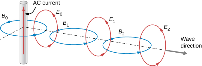
To see how the symmetry introduced by Maxwell accounts for the existence of combined electric and magnetic waves that propagate through space, imagine a time-varying magnetic field [latex]{\stackrel{\to }{\textbf{B}}}_{0}\left(t\right)[/latex] produced by the high-frequency alternating current seen in Figure 16.4. We represent [latex]{\stackrel{\to }{\textbf{B}}}_{0}\left(t\right)[/latex] in the diagram by one of its field lines. From Faraday’s law, the changing magnetic field through a surface induces a time-varying electric field [latex]{\stackrel{\to }{\textbf{E}}}_{0}\left(t\right)[/latex] at the boundary of that surface. The displacement current source for the electric field, like the Faraday’s law source for the magnetic field, produces only closed loops of field lines, because of the mathematical symmetry involved in the equations for the induced electric and induced magnetic fields. A field line representation of [latex]{\stackrel{\to }{\textbf{E}}}_{0}\left(t\right)[/latex] is shown. In turn, the changing electric field [latex]{\stackrel{\to }{\textbf{E}}}_{0}\left(t\right)[/latex] creates a magnetic field [latex]{\stackrel{\to }{\textbf{B}}}_{1}\left(t\right)[/latex] according to the modified Ampère’s law. This changing field induces [latex]{\stackrel{\to }{\textbf{E}}}_{1}\left(t\right),[/latex] which induces [latex]{\stackrel{\to }{\textbf{B}}}_{2}\left(t\right),[/latex] and so on. We then have a self-continuing process that leads to the creation of time-varying electric and magnetic fields in regions farther and farther away from O. This process may be visualized as the propagation of an electromagnetic wave through space.
In the next section, we show in more precise mathematical terms how Maxwell’s equations lead to the prediction of electromagnetic waves that can travel through space without a material medium, implying a speed of electromagnetic waves equal to the speed of light.
Prior to Maxwell’s work, experiments had already indicated that light was a wave phenomenon, although the nature of the waves was yet unknown. In 1801, Thomas Young (1773–1829) showed that when a light beam was separated by two narrow slits and then recombined, a pattern made up of bright and dark fringes was formed on a screen. Young explained this behavior by assuming that light was composed of waves that added constructively at some points and destructively at others (see Interference). Subsequently, Jean Foucault (1819–1868), with measurements of the speed of light in various media, and Augustin Fresnel (1788–1827), with detailed experiments involving interference and diffraction of light, provided further conclusive evidence that light was a wave. So, light was known to be a wave, and Maxwell had predicted the existence of electromagnetic waves that traveled at the speed of light. The conclusion seemed inescapable: Light must be a form of electromagnetic radiation. But Maxwell’s theory showed that other wavelengths and frequencies than those of light were possible for electromagnetic waves. He showed that electromagnetic radiation with the same fundamental properties as visible light should exist at any frequency. It remained for others to test, and confirm, this prediction.
Check Your Understanding
When the emf across a capacitor is turned on and the capacitor is allowed to charge, when does the magnetic field induced by the displacement current have the greatest magnitude?
Show Solution
It is greatest immediately after the current is switched on. The displacement current and the magnetic field from it are proportional to the rate of change of electric field between the plates, which is greatest when the plates first begin to charge.
Hertz’s Observations
The German physicist Heinrich Hertz (1857–1894) was the first to generate and detect certain types of electromagnetic waves in the laboratory. Starting in 1887, he performed a series of experiments that not only confirmed the existence of electromagnetic waves but also verified that they travel at the speed of light.
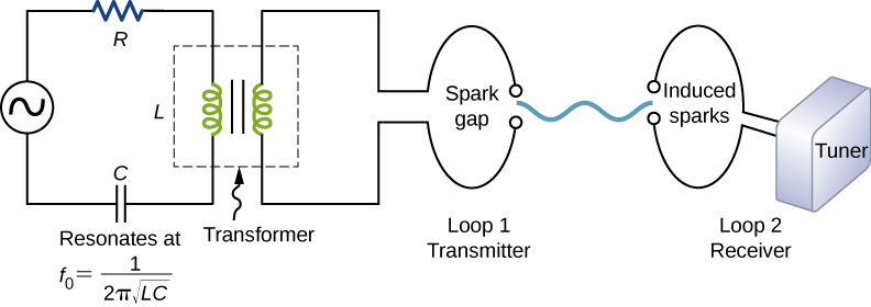
Hertz used an alternating-current RLC (resistor-inductor-capacitor) circuit that resonates at a known frequency [latex]{f}_{0}=\frac{1}{2\text{π}\phantom{\rule{0.2em}{0ex}}\sqrt{LC}}[/latex] and connected it to a loop of wire, as shown in Figure 16.5. High voltages induced across the gap in the loop produced sparks that were visible evidence of the current in the circuit and helped generate electromagnetic waves.
Across the laboratory, Hertz placed another loop attached to another RLC circuit, which could be tuned (as the dial on a radio) to the same resonant frequency as the first and could thus be made to receive electromagnetic waves. This loop also had a gap across which sparks were generated, giving solid evidence that electromagnetic waves had been received.
Hertz also studied the reflection, refraction, and interference patterns of the electromagnetic waves he generated, confirming their wave character. He was able to determine the wavelengths from the interference patterns, and knowing their frequencies, he could calculate the propagation speed using the equation [latex]v=f\lambda[/latex], where v is the speed of a wave, f is its frequency, and [latex]\lambda[/latex] is its wavelength. Hertz was thus able to prove that electromagnetic waves travel at the speed of light. The SI unit for frequency, the hertz ([latex]1\phantom{\rule{0.2em}{0ex}}\text{Hz}=1\phantom{\rule{0.2em}{0ex}}\text{cycle/s}[/latex]), is named in his honor.
Check Your Understanding
Could a purely electric field propagate as a wave through a vacuum without a magnetic field? Justify your answer.
Show Solution
No. The changing electric field according to the modified version of Ampère’s law would necessarily induce a changing magnetic field.
Summary
- Maxwell’s prediction of electromagnetic waves resulted from his formulation of a complete and symmetric theory of electricity and magnetism, known as Maxwell’s equations.
- The four Maxwell’s equations together with the Lorentz force law encompass the major laws of electricity and magnetism. The first of these is Gauss’s law for electricity; the second is Gauss’s law for magnetism; the third is Faraday’s law of induction (including Lenz’s law); and the fourth is Ampère’s law in a symmetric formulation that adds another source of magnetism, namely changing electric fields.
- The symmetry introduced between electric and magnetic fields through Maxwell’s displacement current explains the mechanism of electromagnetic wave propagation, in which changing magnetic fields produce changing electric fields and vice versa.
- Although light was already known to be a wave, the nature of the wave was not understood before Maxwell. Maxwell’s equations also predicted electromagnetic waves with wavelengths and frequencies outside the range of light. These theoretical predictions were first confirmed experimentally by Heinrich Hertz.
Conceptual Questions
Explain how the displacement current maintains the continuity of current in a circuit containing a capacitor.
Show Solution
The current into the capacitor to change the electric field between the plates is equal to the displacement current between the plates.
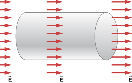
Describe the field lines of the induced magnetic field along the edge of the imaginary horizontal cylinder shown below if the cylinder is in a spatially uniform electric field that is horizontal, pointing to the right, and increasing in magnitude.
Why is it much easier to demonstrate in a student lab that a changing magnetic field induces an electric field than it is to demonstrate that a changing electric field produces a magnetic field?
Show Solution
The first demonstration requires simply observing the current produced in a wire that experiences a changing magnetic field. The second demonstration requires moving electric charge from one location to another, and therefore involves electric currents that generate a changing electric field. The magnetic fields from these currents are not easily separated from the magnetic field that the displacement current produces.
Problems
Show that the magnetic field at a distance r from the axis of two circular parallel plates, produced by placing charge Q(t) on the plates is
[latex]{B}_{\text{ind}}=\frac{{\mu }_{0}}{2\pi r}\phantom{\rule{0.2em}{0ex}}\frac{dQ\left(t\right)}{dt}[/latex].
Show Solution
[latex]\begin{array}{cc}\hfill {B}_{\text{ind}}& =\frac{{\mu }_{0}}{2\pi r}{I}_{\text{ind}}=\frac{{\mu }_{0}}{2\pi r}{\epsilon }_{0}\frac{\partial {\text{Φ}}_{E}}{\partial t}=\frac{{\mu }_{0}}{2\pi r}{\epsilon }_{0}\left(A\frac{\partial E}{\partial t}\right)=\frac{{\mu }_{0}}{2\pi r}{\epsilon }_{0}A\left(\frac{1}{d}\phantom{\rule{0.2em}{0ex}}\frac{dV\left(t\right)}{dt}\right)\hfill \\ & =\frac{{\mu }_{0}}{2\pi r}\left[\frac{{\epsilon }_{0}A}{d}\right]\phantom{\rule{0.2em}{0ex}}\left[\frac{1}{C}\phantom{\rule{0.2em}{0ex}}\frac{dQ\left(t\right)}{dt}\right]=\frac{{\mu }_{0}}{2\pi r}\phantom{\rule{0.2em}{0ex}}\frac{dQ\left(t\right)}{dt}\phantom{\rule{2em}{0ex}}\text{because}\phantom{\rule{0.2em}{0ex}}C=\frac{{\epsilon }_{0}A}{d}\hfill \end{array}[/latex]
Express the displacement current in a capacitor in terms of the capacitance and the rate of change of the voltage across the capacitor.
A potential difference [latex]V\left(t\right)={V}_{0}\phantom{\rule{0.2em}{0ex}}\text{sin}\phantom{\rule{0.2em}{0ex}}\omega t[/latex] is maintained across a parallel-plate capacitor with capacitance C consisting of two circular parallel plates. A thin wire with resistance R connects the centers of the two plates, allowing charge to leak between plates while they are charging.
(a) Obtain expressions for the leakage current [latex]{I}_{\text{res}}\left(t\right)[/latex] in the thin wire. Use these results to obtain an expression for the current [latex]{I}_{\text{real}}\left(t\right)[/latex] in the wires connected to the capacitor.
(b) Find the displacement current in the space between the plates from the changing electric field between the plates.
(c) Compare [latex]{I}_{\text{real}}\left(t\right)[/latex] with the sum of the displacement current [latex]{I}_{\text{d}}\left(t\right)[/latex] and resistor current [latex]{I}_{\text{res}}\left(t\right)[/latex] between the plates, and explain why the relationship you observe would be expected.
Show Solution
a. [latex]{I}_{\text{res}}=\frac{{V}_{0}\phantom{\rule{0.2em}{0ex}}\text{sin}\phantom{\rule{0.2em}{0ex}}\omega t}{R}[/latex]; b. [latex]{I}_{\text{d}}=C{V}_{0}\omega \phantom{\rule{0.2em}{0ex}}\text{cos}\phantom{\rule{0.2em}{0ex}}\omega t[/latex];
c. [latex]{I}_{\text{real}}={I}_{\text{res}}+\frac{dQ}{dt}=\frac{{V}_{0}\phantom{\rule{0.2em}{0ex}}\text{sin}\phantom{\rule{0.2em}{0ex}}\omega t}{R}+C{V}_{0}\frac{d}{dt}\phantom{\rule{0.2em}{0ex}}\text{sin}\phantom{\rule{0.2em}{0ex}}\omega t=\frac{{V}_{0}\phantom{\rule{0.2em}{0ex}}\text{sin}\phantom{\rule{0.2em}{0ex}}\omega t}{R}+C{V}_{0}\omega \phantom{\rule{0.2em}{0ex}}\text{cos}\phantom{\rule{0.2em}{0ex}}\omega t[/latex]; which is the sum of [latex]{I}_{\text{res}}[/latex] and [latex]{I}_{\text{real}},[/latex] consistent with how the displacement current maintaining the continuity of current.
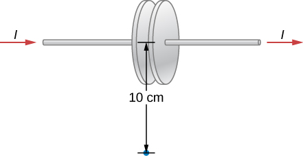
Suppose the parallel-plate capacitor shown below is accumulating charge at a rate of 0.010 C/s. What is the induced magnetic field at a distance of 10 cm from the capacitator?
The potential difference V(t) between parallel plates shown above is instantaneously increasing at a rate of [latex]{10}^{7}\phantom{\rule{0.2em}{0ex}}\text{V/s}.[/latex] What is the displacement current between the plates if the separation of the plates is 1.00 cm and they have an area of [latex]0.200{\phantom{\rule{0.2em}{0ex}}\text{m}}^{2}[/latex] ?
Show Solution
[latex]1.77\phantom{\rule{0.2em}{0ex}}×\phantom{\rule{0.2em}{0ex}}{10}^{-3}\phantom{\rule{0.2em}{0ex}}\text{A}[/latex]
A parallel-plate capacitor has a plate area of [latex]A=0.250{\phantom{\rule{0.2em}{0ex}}\text{m}}^{2}[/latex] and a separation of 0.0100 m. What must be must be the angular frequency [latex]\omega[/latex] for a voltage [latex]V\left(t\right)={V}_{0}\phantom{\rule{0.2em}{0ex}}\text{sin}\phantom{\rule{0.2em}{0ex}}\omega t[/latex] with [latex]{V}_{0}=100\phantom{\rule{0.2em}{0ex}}\text{V}[/latex] to produce a maximum displacement induced current of 1.00 A between the plates?
The voltage across a parallel-plate capacitor with area [latex]A=800{\phantom{\rule{0.2em}{0ex}}\text{cm}}^{2}[/latex] and separation [latex]d=2\phantom{\rule{0.2em}{0ex}}\text{mm}[/latex] varies sinusoidally as [latex]V=\left(15\phantom{\rule{0.2em}{0ex}}\text{mV}\right)\phantom{\rule{0.2em}{0ex}}\text{cos}\phantom{\rule{0.2em}{0ex}}\left(150t\right)[/latex], where t is in seconds. Find the displacement current between the plates.
Show Solution
[latex]{I}_{\text{d}}=\left(7.97\phantom{\rule{0.2em}{0ex}}×\phantom{\rule{0.2em}{0ex}}{10}^{-10}\phantom{\rule{0.2em}{0ex}}\text{A}\right)\phantom{\rule{0.2em}{0ex}}\text{sin}\phantom{\rule{0.2em}{0ex}}\left(150\phantom{\rule{0.2em}{0ex}}t\right)[/latex]
The voltage across a parallel-plate capacitor with area A and separation d varies with time t as [latex]V=a{t}^{2}[/latex], where a is a constant. Find the displacement current between the plates.
Glossary
- displacement current
- extra term in Maxwell’s equations that is analogous to a real current but accounts for a changing electric field producing a magnetic field, even when the real current is present
- Maxwell’s equations
- set of four equations that comprise a complete, overarching theory of electromagnetism
Licenses and Attributions
Maxwell’s Equations and Electromagnetic Waves. Authored by: OpenStax College. Located at: https://openstax.org/books/university-physics-volume-2/pages/16-1-maxwells-equations-and-electromagnetic-waves. License: CC BY: Attribution. License Terms: Download for free at https://openstax.org/books/university-physics-volume-2/pages/1-introduction
