
Chapter 12. Sources of Magnetic Fields
12.6 Solenoids and Toroids
Learning Objectives
By the end of this section, you will be able to:
- Establish a relationship for how the magnetic field of a solenoid varies with distance and current by using both the Biot-Savart law and Ampère’s law
- Establish a relationship for how the magnetic field of a toroid varies with distance and current by using Ampère’s law
Two of the most common and useful electromagnetic devices are called solenoids and toroids. In one form or another, they are part of numerous instruments, both large and small. In this section, we examine the magnetic field typical of these devices.
Solenoids
A long wire wound in the form of a helical coil is known as a solenoid. Solenoids are commonly used in experimental research requiring magnetic fields. A solenoid is generally easy to wind, and near its center, its magnetic field is quite uniform and directly proportional to the current in the wire.
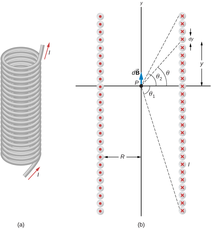
Figure 12.19 shows a solenoid consisting of N turns of wire tightly wound over a length L. A current I is flowing along the wire of the solenoid. The number of turns per unit length is N/L; therefore, the number of turns in an infinitesimal length dy are (N/L)dy turns. This produces a current
We first calculate the magnetic field at the point P of Figure 12.19. This point is on the central axis of the solenoid. We are basically cutting the solenoid into thin slices that are dy thick and treating each as a current loop. Thus, dI is the current through each slice. The magnetic field [latex]d\stackrel{\to }{\textbf{B}}[/latex] due to the current dI in dy can be found with the help of Equation 12.15 and Equation 12.24:
where we used Equation 12.24 to replace dI. The resultant field at P is found by integrating [latex]d\stackrel{\to }{\textbf{B}}[/latex] along the entire length of the solenoid. It’s easiest to evaluate this integral by changing the independent variable from y to [latex]\theta .[/latex] From inspection of Figure 12.19, we have:
Taking the differential of both sides of this equation, we obtain
When this is substituted into the equation for [latex]d\stackrel{\to }{\textbf{B}},[/latex] we have
which is the magnetic field along the central axis of a finite solenoid.
Of special interest is the infinitely long solenoid, for which [latex]L\to \infty .[/latex] From a practical point of view, the infinite solenoid is one whose length is much larger than its radius [latex]\left(L\gg R\right).[/latex] In this case, [latex]{\theta }_{1}=\frac{\text{−}\pi }{2}[/latex] and [latex]{\theta }_{2}=\frac{\pi }{2}.[/latex] Then from Equation 12.27, the magnetic field along the central axis of an infinite solenoid is
or
where n is the number of turns per unit length. You can find the direction of [latex]\stackrel{\to }{\textbf{B}}[/latex] with a right-hand rule: Curl your fingers in the direction of the current, and your thumb points along the magnetic field in the interior of the solenoid.
We now use these properties, along with Ampère’s law, to calculate the magnitude of the magnetic field at any location inside the infinite solenoid. Consider the closed path of Figure 12.20. Along segment 1, [latex]\stackrel{\to }{\textbf{B}}[/latex] is uniform and parallel to the path. Along segments 2 and 4, [latex]\stackrel{\to }{\textbf{B}}[/latex] is perpendicular to part of the path and vanishes over the rest of it. Therefore, segments 2 and 4 do not contribute to the line integral in Ampère’s law. Along segment 3, [latex]\stackrel{\to }{\textbf{B}}=0[/latex] because the magnetic field is zero outside the solenoid. If you consider an Ampère’s law loop outside of the solenoid, the current flows in opposite directions on different segments of wire. Therefore, there is no enclosed current and no magnetic field according to Ampère’s law. Thus, there is no contribution to the line integral from segment 3. As a result, we find
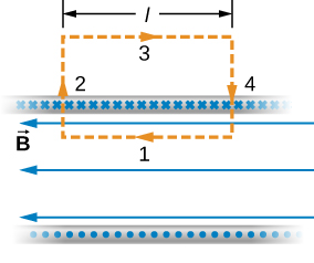
The solenoid has n turns per unit length, so the current that passes through the surface enclosed by the path is nlI. Therefore, from Ampère’s law,
and
within the solenoid. This agrees with what we found earlier for B on the central axis of the solenoid. Here, however, the location of segment 1 is arbitrary, so we have found that this equation gives the magnetic field everywhere inside the infinite solenoid.
Outside the solenoid, one can draw an Ampère’s law loop around the entire solenoid. This would enclose current flowing in both directions. Therefore, the net current inside the loop is zero. According to Ampère’s law, if the net current is zero, the magnetic field must be zero. Therefore, for locations outside of the solenoid’s radius, the magnetic field is zero.
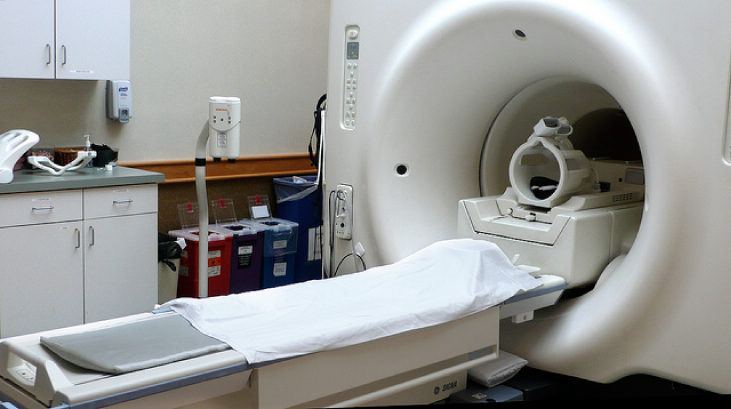
When a patient undergoes a magnetic resonance imaging (MRI) scan, the person lies down on a table that is moved into the center of a large solenoid that can generate very large magnetic fields. The solenoid is capable of these high fields from high currents flowing through superconducting wires. The large magnetic field is used to change the spin of protons in the patient’s body. The time it takes for the spins to align or relax (return to original orientation) is a signature of different tissues that can be analyzed to see if the structures of the tissues is normal (Figure 12.21).
Example
Magnetic Field Inside a Solenoid
A solenoid has 300 turns wound around a cylinder of diameter 1.20 cm and length 14.0 cm. If the current through the coils is 0.410 A, what is the magnitude of the magnetic field inside and near the middle of the solenoid?
Strategy
We are given the number of turns and the length of the solenoid so we can find the number of turns per unit length. Therefore, the magnetic field inside and near the middle of the solenoid is given by Equation 12.30. Outside the solenoid, the magnetic field is zero.
Solution
Show Answer
The number of turns per unit length is
The magnetic field produced inside the solenoid is
Significance
This solution is valid only if the length of the solenoid is reasonably large compared with its diameter. This example is a case where this is valid.
Check Your Understanding
What is the ratio of the magnetic field produced from using a finite formula over the infinite approximation for an angle [latex]\theta[/latex] of (a) [latex]85\text{°}\text{?}[/latex] (b) [latex]89\text{°}\text{?}[/latex] The solenoid has 1000 turns in 50 cm with a current of 1.0 A flowing through the coils
Show Solution
a. 1.00382; b. 1.00015
Toroids
A toroid is a donut-shaped coil closely wound with one continuous wire, as illustrated in part (a) of Figure 12.22. If the toroid has N windings and the current in the wire is I, what is the magnetic field both inside and outside the toroid?
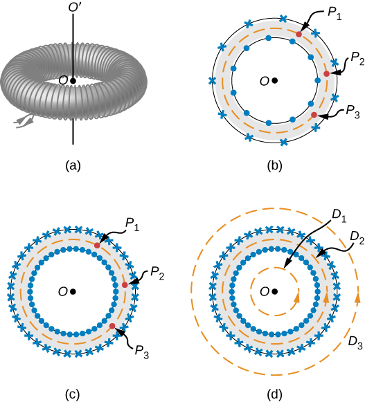
We begin by assuming cylindrical symmetry around the axis OO’. Actually, this assumption is not precisely correct, for as part (b) of Figure 12.22 shows, the view of the toroidal coil varies from point to point (for example, [latex]{P}_{1},\phantom{\rule{0.2em}{0ex}}{P}_{2},[/latex] and [latex]{P}_{3}[/latex]) on a circular path centered around OO’. However, if the toroid is tightly wound, all points on the circle become essentially equivalent [part (c) of Figure 12.22], and cylindrical symmetry is an accurate approximation.
With this symmetry, the magnetic field must be tangent to and constant in magnitude along any circular path centered on OO’. This allows us to write for each of the paths [latex]{D}_{1},{D}_{2},[/latex] and [latex]{D}_{3}[/latex] shown in part (d) of Figure 12.22,
Ampère’s law relates this integral to the net current passing through any surface bounded by the path of integration. For a path that is external to the toroid, either no current passes through the enclosing surface (path [latex]{D}_{1}[/latex]), or the current passing through the surface in one direction is exactly balanced by the current passing through it in the opposite direction [latex]\left(\text{path}\phantom{\rule{0.2em}{0ex}}{D}_{3}\right).[/latex] In either case, there is no net current passing through the surface, so
and
The turns of a toroid form a helix, rather than circular loops. As a result, there is a small field external to the coil; however, the derivation above holds if the coils were circular.
For a circular path within the toroid (path [latex]{D}_{2}[/latex]), the current in the wire cuts the surface N times, resulting in a net current NI through the surface. We now find with Ampère’s law,
and
The magnetic field is directed in the counterclockwise direction for the windings shown. When the current in the coils is reversed, the direction of the magnetic field also reverses.
The magnetic field inside a toroid is not uniform, as it varies inversely with the distance r from the axis OO’. However, if the central radius R (the radius midway between the inner and outer radii of the toroid) is much larger than the cross-sectional diameter of the coils r, the variation is fairly small, and the magnitude of the magnetic field may be calculated by Equation 12.33 where [latex]r=R.[/latex]
Summary
- The magnetic field strength inside a solenoid is
[latex]B={\mu }_{0}nI\phantom{\rule{1em}{0ex}}\text{(inside a solenoid)}[/latex]
where n is the number of loops per unit length of the solenoid. The field inside is very uniform in magnitude and direction. - The magnetic field strength inside a toroid is
[latex]B=\frac{{\mu }_{o}NI}{2\pi r}\phantom{\rule{1em}{0ex}}\text{(within the toroid)}[/latex]
where N is the number of windings. The field inside a toroid is not uniform and varies with the distance as 1/r.
Conceptual Questions
Is the magnetic field inside a toroid completely uniform? Almost uniform?
Explain why [latex]\stackrel{\to }{\textbf{B}}=0[/latex] inside a long, hollow copper pipe that is carrying an electric current parallel to the axis. Is [latex]\stackrel{\to }{\textbf{B}}=0[/latex] outside the pipe?
Show Solution
If there is no current inside the loop, there is no magnetic field (see Ampère’s law). Outside the pipe, there may be an enclosed current through the copper pipe, so the magnetic field may not be zero outside the pipe.
Problems
A solenoid is wound with 2000 turns per meter. When the current is 5.2 A, what is the magnetic field within the solenoid?
Show Solution
[latex]B=1.3\phantom{\rule{0.2em}{0ex}}×\phantom{\rule{0.2em}{0ex}}{10}^{-2}\text{T}[/latex]
A solenoid has 12 turns per centimeter. What current will produce a magnetic field of [latex]2.0\phantom{\rule{0.2em}{0ex}}×\phantom{\rule{0.2em}{0ex}}{10}^{-2}\text{T}[/latex] within the solenoid?
If a current is 2.0 A, how many turns per centimeter must be wound on a solenoid in order to produce a magnetic field of [latex]2.0\phantom{\rule{0.2em}{0ex}}×\phantom{\rule{0.2em}{0ex}}{10}^{-3}\text{T}[/latex] within it?
Show Solution
roughly eight turns per cm
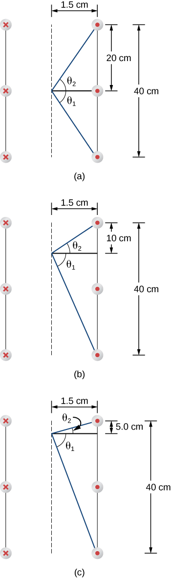
A solenoid is 40 cm long, has a diameter of 3.0 cm, and is wound with 500 turns. If the current through the windings is 4.0 A, what is the magnetic field at a point on the axis of the solenoid that is (a) at the center of the solenoid, (b) 10.0 cm from one end of the solenoid, and (c) 5.0 cm from one end of the solenoid? (d) Compare these answers with the infinite-solenoid case.
Determine the magnetic field on the central axis at the opening of a semi-infinite solenoid. (That is, take the opening to be at [latex]x=0[/latex] and the other end to be at
[latex]x=\infty .[/latex])
Show Solution
[latex]B=\frac{1}{2}{\mu }_{0}nI[/latex]
By how much is the approximation [latex]B={\mu }_{0}nI[/latex] in error at the center of a solenoid that is 15.0 cm long, has a diameter of 4.0 cm, is wrapped with n turns per meter, and carries a current I?
A solenoid with 25 turns per centimeter carries a current I. An electron moves within the solenoid in a circle that has a radius of 2.0 cm and is perpendicular to the axis of the solenoid. If the speed of the electron is [latex]2.0\phantom{\rule{0.2em}{0ex}}×\phantom{\rule{0.2em}{0ex}}{10}^{5}\text{m/s},[/latex] what is I?
Show Solution
0.0181 A
A toroid has 250 turns of wire and carries a current of 20 A. Its inner and outer radii are 8.0 and 9.0 cm. What are the values of its magnetic field at [latex]r=8.1,8.5,[/latex] and [latex]8.9\phantom{\rule{0.2em}{0ex}}\text{cm?}[/latex]
A toroid with a square cross section 3.0 cm [latex]\phantom{\rule{0.2em}{0ex}}×\phantom{\rule{0.2em}{0ex}}[/latex] 3.0 cm has an inner radius of 25.0 cm. It is wound with 500 turns of wire, and it carries a current of 2.0 A. What is the strength of the magnetic field at the center of the square cross section?
Show Solution
0.0008 T
Glossary
- solenoid
- thin wire wound into a coil that produces a magnetic field when an electric current is passed through it
- toroid
- donut-shaped coil closely wound around that is one continuous wire
Licenses and Attributions
Solenoids and Toroids. Authored by: OpenStax College. Located at: https://openstax.org/books/university-physics-volume-2/pages/12-6-solenoids-and-toroids. License: CC BY: Attribution. License Terms: Download for free at https://openstax.org/books/university-physics-volume-2/pages/1-introduction
