
Chapter 5. Electric Charges and Fields
5.6 Electric Field Lines
Learning Objectives
By the end of this section, you will be able to:
- Explain the purpose of an electric field diagram
- Describe the relationship between a vector diagram and a field line diagram
- Explain the rules for creating a field diagram and why these rules make physical sense
- Sketch the field of an arbitrary source charge
Now that we have some experience calculating electric fields, let’s try to gain some insight into the geometry of electric fields. As mentioned earlier, our model is that the charge on an object (the source charge) alters space in the region around it in such a way that when another charged object (the test charge) is placed in that region of space, that test charge experiences an electric force. The concept of electric field lines, and of electric field line diagrams, enables us to visualize the way in which the space is altered, allowing us to visualize the field. The purpose of this section is to enable you to create sketches of this geometry, so we will list the specific steps and rules involved in creating an accurate and useful sketch of an electric field.
It is important to remember that electric fields are three-dimensional. Although in this book we include some pseudo-three-dimensional images, several of the diagrams that you’ll see (both here, and in subsequent chapters) will be two-dimensional projections, or cross-sections. Always keep in mind that in fact, you’re looking at a three-dimensional phenomenon.
Our starting point is the physical fact that the electric field of the source charge causes a test charge in that field to experience a force. By definition, electric field vectors point in the same direction as the electric force that a (hypothetical) positive test charge would experience, if placed in the field (Figure 5.27)
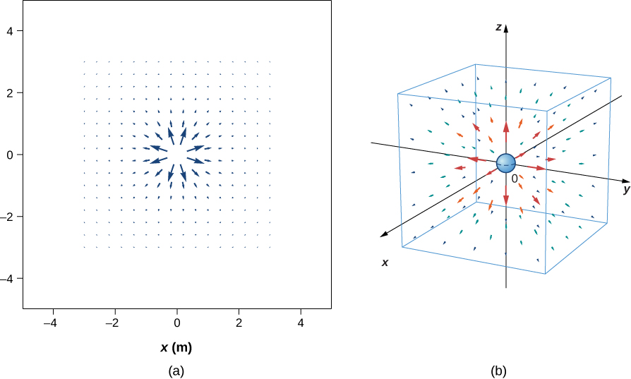
We’ve plotted many field vectors in the figure, which are distributed uniformly around the source charge. Since the electric field is a vector, the arrows that we draw correspond at every point in space to both the magnitude and the direction of the field at that point. As always, the length of the arrow that we draw corresponds to the magnitude of the field vector at that point. For a point source charge, the length decreases by the square of the distance from the source charge. In addition, the direction of the field vector is radially away from the source charge, because the direction of the electric field is defined by the direction of the force that a positive test charge would experience in that field. (Again, keep in mind that the actual field is three-dimensional; there are also field lines pointing out of and into the page.)
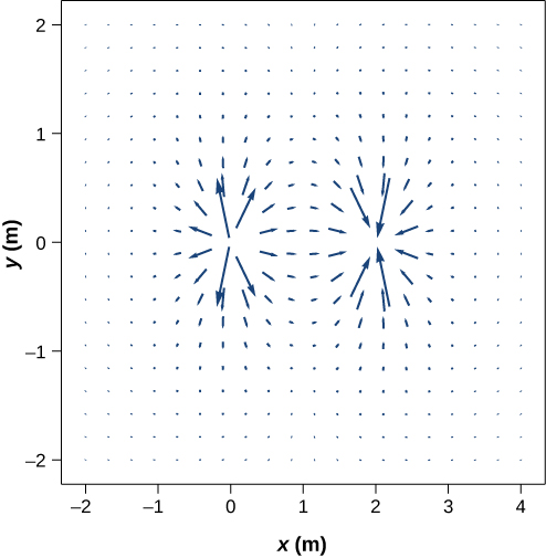
This diagram is correct, but it becomes less useful as the source charge distribution becomes more complicated. For example, consider the vector field diagram of a dipole (Figure 5.28).
There is a more useful way to present the same information. Rather than drawing a large number of increasingly smaller vector arrows, we instead connect all of them together, forming continuous lines and curves, as shown in Figure 5.29.
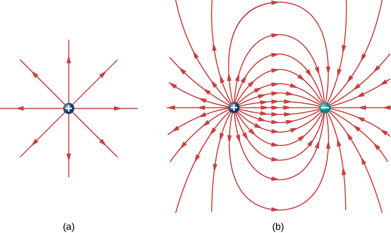
Although it may not be obvious at first glance, these field diagrams convey the same information about the electric field as do the vector diagrams. First, the direction of the field at every point is simply the direction of the field vector at that same point. In other words, at any point in space, the field vector at each point is tangent to the field line at that same point. The arrowhead placed on a field line indicates its direction.
As for the magnitude of the field, that is indicated by the field line density—that is, the number of field lines per unit area passing through a small cross-sectional area perpendicular to the electric field. This field line density is drawn to be proportional to the magnitude of the field at that cross-section. As a result, if the field lines are close together (that is, the field line density is greater), this indicates that the magnitude of the field is large at that point. If the field lines are far apart at the cross-section, this indicates the magnitude of the field is small. Figure 5.30 shows the idea.
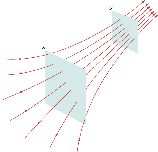
In Figure 5.30, the same number of field lines passes through both surfaces (S and [latex]S\text{′}[/latex]), but the surface S is larger than surface [latex]S\text{′}[/latex]. Therefore, the density of field lines (number of lines per unit area) is larger at the location of [latex]S\text{′}[/latex], indicating that the electric field is stronger at the location of [latex]S\text{′}[/latex] than at S. The rules for creating an electric field diagram are as follows.
Problem-Solving Strategy: Drawing Electric Field Lines
- Electric field lines either originate on positive charges or come in from infinity, and either terminate on negative charges or extend out to infinity.
- The number of field lines originating or terminating at a charge is proportional to the magnitude of that charge. A charge of 2q will have twice as many lines as a charge of q.
- At every point in space, the field vector at that point is tangent to the field line at that same point.
- The field line density at any point in space is proportional to (and therefore is representative of) the magnitude of the field at that point in space.
- Field lines can never cross. Since a field line represents the direction of the field at a given point, if two field lines crossed at some point, that would imply that the electric field was pointing in two different directions at a single point. This in turn would suggest that the (net) force on a test charge placed at that point would point in two different directions. Since this is obviously impossible, it follows that field lines must never cross.
Always keep in mind that field lines serve only as a convenient way to visualize the electric field; they are not physical entities. Although the direction and relative intensity of the electric field can be deduced from a set of field lines, the lines can also be misleading. For example, the field lines drawn to represent the electric field in a region must, by necessity, be discrete. However, the actual electric field in that region exists at every point in space.
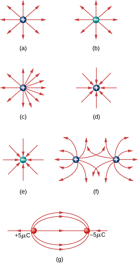
Field lines for three groups of discrete charges are shown in Figure 5.31. Since the charges in parts (a) and (b) have the same magnitude, the same number of field lines are shown starting from or terminating on each charge. In (c), however, we draw three times as many field lines leaving the [latex]\text{+}3q[/latex] charge as entering the [latex]\text{−}q[/latex]. The field lines that do not terminate at [latex]\text{−}q[/latex] emanate outward from the charge configuration, to infinity.

The ability to construct an accurate electric field diagram is an important, useful skill; it makes it much easier to estimate, predict, and therefore calculate the electric field of a source charge. The best way to develop this skill is with software that allows you to place source charges and then will draw the net field upon request. We strongly urge you to search the Internet for a program. Once you’ve found one you like, run several simulations to get the essential ideas of field diagram construction. Then practice drawing field diagrams, and checking your predictions with the computer-drawn diagrams.
One example of a field-line drawing program is from the PhET “Charges and Fields” simulation.
Summary
- Electric field diagrams assist in visualizing the field of a source charge.
- The magnitude of the field is proportional to the field line density.
- Field vectors are everywhere tangent to field lines.
Conceptual Questions
If a point charge is released from rest in a uniform electric field, will it follow a field line? Will it do so if the electric field is not uniform?
Show Solution
yes; no
Under what conditions, if any, will the trajectory of a charged particle not follow a field line?
How would you experimentally distinguish an electric field from a gravitational field?
Show Solution
At the surface of Earth, the gravitational field is always directed in toward Earth’s center. An electric field could move a charged particle in a different direction than toward the center of Earth. This would indicate an electric field is present.
A representation of an electric field shows 10 field lines perpendicular to a square plate. How many field lines should pass perpendicularly through the plate to depict a field with twice the magnitude?
What is the ratio of the number of electric field lines leaving a charge 10q and a charge q?
Show Solution
10
Problems
Which of the following electric field lines are incorrect for point charges? Explain why.
In this exercise, you will practice drawing electric field lines. Make sure you represent both the magnitude and direction of the electric field adequately. Note that the number of lines into or out of charges is proportional to the charges.
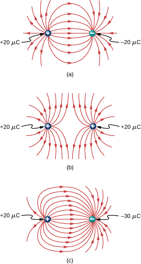
(a) Draw the electric field lines map for two charges [latex]\text{+}20\phantom{\rule{0.2em}{0ex}}\mu \text{C}[/latex] and [latex]-20\phantom{\rule{0.2em}{0ex}}\mu \text{C}[/latex] situated 5 cm from each other.
(b) Draw the electric field lines map for two charges [latex]\text{+}20\phantom{\rule{0.2em}{0ex}}\mu \text{C}[/latex] and [latex]\text{+}20\phantom{\rule{0.2em}{0ex}}\mu \text{C}[/latex] situated 5 cm from each other.
(c) Draw the electric field lines map for two charges [latex]\text{+}20\phantom{\rule{0.2em}{0ex}}\mu \text{C}[/latex] and [latex]-30\phantom{\rule{0.2em}{0ex}}\mu \text{C}[/latex] situated 5 cm from each other.
Show Solution
Draw the electric field for a system of three particles of charges [latex]\text{+}1\phantom{\rule{0.2em}{0ex}}\mu \text{C},[/latex] [latex]\text{+}2\phantom{\rule{0.2em}{0ex}}\mu \text{C},[/latex] and [latex]-3\phantom{\rule{0.2em}{0ex}}\mu \text{C}[/latex] fixed at the corners of an equilateral triangle of side 2 cm.
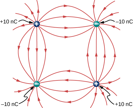
Two charges of equal magnitude but opposite sign make up an electric dipole. A quadrupole consists of two electric dipoles are placed anti-parallel at two edges of a square as shown.
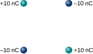
Draw the electric field of the charge distribution.
Show Solution
Suppose the electric field of an isolated point charge decreased with distance as [latex]1\text{/}{r}^{2+\delta }[/latex] rather than as [latex]1\text{/}{r}^{2}[/latex]. Show that it is then impossible to draw continous field lines so that their number per unit area is proportional to E.
Glossary
- field line
- smooth, usually curved line that indicates the direction of the electric field
- field line density
- number of field lines per square meter passing through an imaginary area; its purpose is to indicate the field strength at different points in space
Licenses and Attributions
Electric Field Lines. Authored by: OpenStax College. Located at: https://openstax.org/books/university-physics-volume-2/pages/5-6-electric-field-lines. License: CC BY: Attribution. License Terms: Download for free at https://openstax.org/books/university-physics-volume-2/pages/1-introduction
