2.4 Distribution of Molecular Speeds

Samuel J. Ling; William Moebs; Jeff Sanny

Chapter 2. The Kinetic Theory of Gases

2.4 Distribution of Molecular Speeds

Learning Objectives

By the end of this section, you will be able to:

Describe the distribution of molecular speeds in an ideal gas
Find the average and most probable molecular speeds in an ideal gas

Particles in an ideal gas all travel at relatively high speeds, but they do not travel at the same speed. The rms speed is one kind of average, but many particles move faster and many move slower. The actual distribution of speeds has several interesting implications for other areas of physics, as we will see in later chapters.

The Maxwell-Boltzmann Distribution

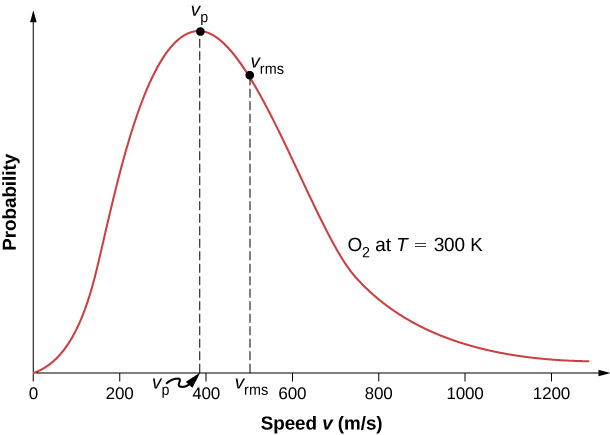
The motion of molecules in a gas is random in magnitude and direction for individual molecules, but a gas of many molecules has a predictable distribution of molecular speeds. This predictable distribution of molecular speeds is known as the Maxwell-Boltzmann distribution, after its originators, who calculated it based on kinetic theory, and it has since been confirmed experimentally (Figure 2.15).

To understand this figure, we must define a distribution function of molecular speeds, since with a finite number of molecules, the probability that a molecule will have exactly a given speed is 0.

The figure is a graph of probability versus velocity v in meters per second of oxygen gas at 300 kelvin. The graph has a peak probability at a velocity V p of just under 400 meters per second and a root-mean-square probability at a velocity v r m s of about 500 meters per second. The probability is zero at the origin and tends to zero at infinity. The graph is not symmetric, but rather steeper on the left than on the right of the peak. — **Figure 2.15** The Maxwell-Boltzmann distribution of molecular speeds in an ideal gas. The most likely speed $v_{p}$ is less than the rms speed $v_{rms}$ . Although very high speeds are possible, only a tiny fraction of the molecules have speeds that are an order of magnitude greater than $v_{rms} .$

We define the distribution function $f (v)$ by saying that the expected number $N (v_{1}, v_{2})$ of particles with speeds between $v_{1}$ and $v_{2}$ is given by

N (v_{1}, v_{2}) = N \int_{v_{1}}^{v_{2}} f (v) d v .

[Since N is dimensionless, the unit of f(v) is seconds per meter.] We can write this equation conveniently in differential form:

d N = N f (v) d v .

In this form, we can understand the equation as saying that the number of molecules with speeds between v and $v + d v$ is the total number of molecules in the sample times f(v) times dv. That is, the probability that a molecule’s speed is between v and $v + d v$ is f(v)dv.

We can now quote Maxwell’s result, although the proof is beyond our scope.

Maxwell-Boltzmann Distribution of Speeds

The distribution function for speeds of particles in an ideal gas at temperature T is

f (v) = \frac{4}{\sqrt{π}} {(\frac{m}{2 k_{B} T})}^{3 / 2} v^{2} e^{− m v^{2} / 2 k_{B} T} .

The factors before the $v^{2}$ are a normalization constant; they make sure that $N (0, \infty) = N$ by making sure that $\int_{0}^{\infty} f (v) d v = 1.$ Let’s focus on the dependence on v. The factor of $v^{2}$ means that $f (0) = 0$ and for small v, the curve looks like a parabola. The factor of $e^{− m_{0} v^{2} / 2 k_{B} T}$ means that $lim_{v \to \infty} f (v) = 0$ and the graph has an exponential tail, which indicates that a few molecules may move at several times the rms speed. The interaction of these factors gives the function the single-peaked shape shown in the figure.

Example

Calculating the Ratio of Numbers of Molecules Near Given Speeds

In a sample of nitrogen ( $N_{2},$ with a molar mass of 28.0 g/mol) at a temperature of $273 °C$ , find the ratio of the number of molecules with a speed very close to 300 m/s to the number with a speed very close to 100 m/s.

Strategy

Since we’re looking at a small range, we can approximate the number of molecules near 100 m/s as $d N_{100} = f (100 m/s) d v .$ Then the ratio we want is

\frac{d N_{300}}{d N_{100}} = \frac{f (300 m/s) d v}{f (100 m/s) d v} = \frac{f (300 m/s)}{f (100 m/s)} .

All we have to do is take the ratio of the two f values.

Solution

Show Answer

Identify the knowns and convert to SI units if necessary.

T = 300 K, k_{B} = 1.38 \times 10^{- 23} J/K

M = 0.0280 kg/mol so m = 4.65 \times 10^{- 26} kg

Substitute the values and solve.

\begin{array}{cc} \frac{f (300 m/s)}{f (100 m/s)} & = \frac{\frac{4}{\sqrt{π}} {(\frac{m}{2 k_{B} T})}^{3 / 2} {(300 m/s)}^{2} exp [− m {(300 m/s)}^{2} / 2 k_{B} T]}{\frac{4}{\sqrt{π}} {(\frac{m}{2 k_{B} T})}^{3 / 2} {(100 m/s)}^{2} exp [− m {(100 m/s)}^{2} / 2 k_{B} T]} \\ = \frac{{(300 m/s)}^{2} exp [− (4.65 \times 10^{- 26} kg) {(300 m/s)}^{2} / 2 (1.38 \times 10^{- 23} J/K) (300 K)]}{{(100 m/s)}^{2} exp [− (4.65 \times 10^{- 26} kg) {(100 m/s)}^{2} / 2 (1.38 \times 10^{- 23} J/K) (300 K)]} \\ = 3^{2} exp [- \frac{(4.65 \times 10^{- 26} kg) [{(300 m/s)}^{2} - {(100 ms)}^{2}]}{2 (1.38 \times 10^{- 23} J/K) (300 K)}] \\ = 5.74 \end{array}

Figure 2.16 shows that the curve is shifted to higher speeds at higher temperatures, with a broader range of speeds.

Two distributions of probability versus velocity v in meters per second at two different temperatures, T one and T two, are plotted on the same graph. Temperature two is greater than Temperature one. The distribution for T two has a broader peak with a maximum at a higher velocity and lower probability than the distribution for Temperature one. — **Figure 2.16** The Maxwell-Boltzmann distribution is shifted to higher speeds and broadened at higher temperatures.

With only a relatively small number of molecules, the distribution of speeds fluctuates around the Maxwell-Boltzmann distribution. However, you can view this simulation to see the essential features that more massive molecules move slower and have a narrower distribution. Use the set-up “2 Gases, Random Speeds”. Note the display at the bottom comparing histograms of the speed distributions with the theoretical curves.

We can use a probability distribution to calculate average values by multiplying the distribution function by the quantity to be averaged and integrating the product over all possible speeds. (This is analogous to calculating averages of discrete distributions, where you multiply each value by the number of times it occurs, add the results, and divide by the number of values. The integral is analogous to the first two steps, and the normalization is analogous to dividing by the number of values.) Thus the average velocity is

\overset{―}{v} = \int_{0}^{\infty} v f (v) d v = \sqrt{\frac{8}{π} \frac{k_{B} T}{m}} = \sqrt{\frac{8}{π} \frac{R T}{M} .}

Similarly,

v_{rms} = \sqrt{\overset{–}{v^{2}}} = \sqrt{\int_{0}^{\infty} v^{2} f (v) d v} = \sqrt{\frac{3 k_{B} T}{m}} = \sqrt{\frac{3 R T}{M}}

as in Pressure, Temperature, and RMS Speed. The most probable speed, also called the peak speed $v_{p},$ is the speed at the peak of the velocity distribution. (In statistics it would be called the mode.) It is less than the rms speed $v_{rms} .$ The most probable speed can be calculated by the more familiar method of setting the derivative of the distribution function, with respect to v, equal to 0. The result is

v_{p} = \sqrt{\frac{2 k_{B} T}{m}} = \sqrt{\frac{2 R T}{M}},

which is less than $v_{rms} .$ In fact, the rms speed is greater than both the most probable speed and the average speed.

The peak speed provides a sometimes more convenient way to write the Maxwell-Boltzmann distribution function:

f (v) = \frac{4 v^{2}}{\sqrt{π} v_{p}^{3}} e^{− v^{2} / v_{p}^{2}}

In the factor $e^{− m v^{2} / 2 k_{B} T}$ , it is easy to recognize the translational kinetic energy. Thus, that expression is equal to $e^{− K / k_{B} T} .$ The distribution f(v) can be transformed into a kinetic energy distribution by requiring that $f (K) d K = f (v) d v .$ Boltzmann showed that the resulting formula is much more generally applicable if we replace the kinetic energy of translation with the total mechanical energy E. Boltzmann’s result is

f (E) = \frac{2}{\sqrt{π}} {(k_{B} T)}^{- 3 / 2} \sqrt{E} e^{− E / k_{B} T} = \frac{2}{\sqrt{π} {(k_{B} T)}^{3 / 2}} \frac{\sqrt{E}}{e^{E / k_{B} T}} .

The first part of this equation, with the negative exponential, is the usual way to write it. We give the second part only to remark that $e^{E / k_{B} T}$ in the denominator is ubiquitous in quantum as well as classical statistical mechanics.

Problem-Solving Strategy: Speed Distribution

Step 1. Examine the situation to determine that it relates to the distribution of molecular speeds.

Step 2. Make a list of what quantities are given or can be inferred from the problem as stated (identify the known quantities).

Step 3. Identify exactly what needs to be determined in the problem (identify the unknown quantities). A written list is useful.

Step 4. Convert known values into proper SI units (K for temperature, Pa for pressure, $m^{3}$ for volume, molecules for N, and moles for n). In many cases, though, using R and the molar mass will be more convenient than using $k_{B}$ and the molecular mass.

Step 5. Determine whether you need the distribution function for velocity or the one for energy, and whether you are using a formula for one of the characteristic speeds (average, most probably, or rms), finding a ratio of values of the distribution function, or approximating an integral.

Step 6. Solve the appropriate equation for the ideal gas law for the quantity to be determined (the unknown quantity). Note that if you are taking a ratio of values of the distribution function, the normalization factors divide out. Or if approximating an integral, use the method asked for in the problem.

Step 7. Substitute the known quantities, along with their units, into the appropriate equation and obtain numerical solutions complete with units.

We can now gain a qualitative understanding of a puzzle about the composition of Earth’s atmosphere. Hydrogen is by far the most common element in the universe, and helium is by far the second-most common. Moreover, helium is constantly produced on Earth by radioactive decay. Why are those elements so rare in our atmosphere? The answer is that gas molecules that reach speeds above Earth’s escape velocity, about 11 km/s, can escape from the atmosphere into space. Because of the lower mass of hydrogen and helium molecules, they move at higher speeds than other gas molecules, such as nitrogen and oxygen. Only a few exceed escape velocity, but far fewer heavier molecules do. Thus, over the billions of years that Earth has existed, far more hydrogen and helium molecules have escaped from the atmosphere than other molecules, and hardly any of either is now present.

We can also now take another look at evaporative cooling, which we discussed in the chapter on temperature and heat. Liquids, like gases, have a distribution of molecular energies. The highest-energy molecules are those that can escape from the intermolecular attractions of the liquid. Thus, when some liquid evaporates, the molecules left behind have a lower average energy, and the liquid has a lower temperature.

Summary

The motion of individual molecules in a gas is random in magnitude and direction. However, a gas of many molecules has a predictable distribution of molecular speeds, known as the Maxwell-Boltzmann distribution.
The average and most probable velocities of molecules having the Maxwell-Boltzmann speed distribution, as well as the rms velocity, can be calculated from the temperature and molecular mass.

Key Equations

Ideal gas law in terms of molecules

p V = N k_{B} T

Ideal gas law ratios if the amount of gas is constant

\frac{p_{1} V_{1}}{T_{1}} = \frac{p_{2} V_{2}}{T_{2}}

Ideal gas law in terms of moles

p V = n R T

Van der Waals equation

[p + a {(\frac{n}{V})}^{2}] (V − n b) = n R T

Pressure, volume, and molecular speed

p V = ​ \frac{1}{3} N m \overset{–}{v^{2}}

Root-mean-square speed

v_{rms} = \sqrt{\frac{3 R T}{M}} = \sqrt{\frac{3 k_{B} T}{m}}

Mean free path

λ = \frac{V}{4 \sqrt{2} π r^{2} N} = \frac{k_{B} T}{4 \sqrt{2} π r^{2} p}

Mean free time

τ = \frac{k_{B} T}{4 \sqrt{2} π r^{2} p v_{rms}}

The following two equations apply only to a monatomic ideal gas:

Average kinetic energy of a molecule

\overset{–}{K} = \frac{3}{2} k_{B} T

Internal energy

E_{int} = \frac{3}{2} N k_{B} T .

Heat in terms of molar heat capacity at constant volume

Q = n C_{V} Δ T

Molar heat capacity at constant volume for an ideal gas with d degrees of freedom

C_{V} = \frac{d}{2} R

Maxwell–Boltzmann speed distribution

f (v) = \frac{4}{\sqrt{π}} {(\frac{m}{2 k_{B} T})}^{3 / 2} v^{2} e^{− m v^{2} / 2 k_{B} T}

Average velocity of a molecule

\overset{―}{v} = \sqrt{\frac{8}{π} \frac{k_{B} T}{m}} = \sqrt{\frac{8}{π} \frac{R T}{M}}

Peak velocity of a molecule

v_{p} = \sqrt{\frac{2 k_{B} T}{m}} = \sqrt{\frac{2 R T}{M}}

Conceptual Questions

One cylinder contains helium gas and another contains krypton gas at the same temperature. Mark each of these statements true, false, or impossible to determine from the given information. (a) The rms speeds of atoms in the two gases are the same. (b) The average kinetic energies of atoms in the two gases are the same. (c) The internal energies of 1 mole of gas in each cylinder are the same. (d) The pressures in the two cylinders are the same.

Show Solution

a. false; b. true; c. true; d. true

Repeat the previous question if one gas is still helium but the other is changed to fluorine, $F_{2}$ .

An ideal gas is at a temperature of 300 K. To double the average speed of its molecules, what does the temperature need to be changed to?

Show Solution

1200 K

Problems

In a sample of hydrogen sulfide $(M = 34.1 g/mol)$ at a temperature of $3.00 \times 10^{2} K,$ estimate the ratio of the number of molecules that have speeds very close to $v_{rms}$ to the number that have speeds very close to $2 v_{rms} .$

Using the approximation $\int_{v_{1}}^{v_{1} + Δ v} f (v) d v \approx f (v_{1}) Δ v$ for small $Δ v$ , estimate the fraction of nitrogen molecules at a temperature of $3.00 \times 10^{2} K$ that have speeds between 290 m/s and 291 m/s.

Show Solution

0.00157

Using the method of the preceding problem, estimate the fraction of nitric oxide (NO) molecules at a temperature of 250 K that have energies between $3.45 \times 10^{- 21} J$ and $3.50 \times 10^{- 21} J$ .

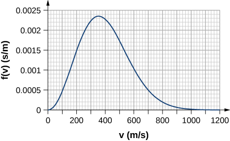
By counting squares in the following figure, estimate the fraction of argon atoms at $T = 300 K$ that have speeds between 600 m/s and 800 m/s. The curve is correctly normalized. The value of a square is its length as measured on the x-axis times its height as measured on the y-axis, with the units given on those axes.

Show Solution

About 0.072. Answers may vary slightly. A more accurate answer is 0.074.

Using a numerical integration method such as Simpson’s rule, find the fraction of molecules in a sample of oxygen gas at a temperature of 250 K that have speeds between 100 m/s and 150 m/s. The molar mass of oxygen $(O_{2})$ is 32.0 g/mol. A precision to two significant digits is enough.

Find (a) the most probable speed, (b) the average speed, and (c) the rms speed for nitrogen molecules at 295 K.

Show Solution

a. 419 m/s; b. 472 m/s; c. 513 m/s

Repeat the preceding problem for nitrogen molecules at 2950 K.

At what temperature is the average speed of carbon dioxide molecules $(M = 44.0 g/mol)$ 510 m/s?

Show Solution

541 K

The most probable speed for molecules of a gas at 296 K is 263 m/s. What is the molar mass of the gas? (You might like to figure out what the gas is likely to be.)

a) At what temperature do oxygen molecules have the same average speed as helium atoms $(M = 4.00 g/mol)$ have at 300 K? b) What is the answer to the same question about most probable speeds? c) What is the answer to the same question about rms speeds?

Show Solution

2400 K for all three parts

Additional Problems

In the deep space between galaxies, the density of molecules (which are mostly single atoms) can be as low as $10^{6} {atoms/m}^{3},$ and the temperature is a frigid 2.7 K. What is the pressure? (b) What volume (in $m^{3}$ ) is occupied by 1 mol of gas? (c) If this volume is a cube, what is the length of its sides in kilometers?

(a) Find the density in SI units of air at a pressure of 1.00 atm and a temperature of $20 °C$ , assuming that air is $78 N_{2}, 21 O_{2}, and 1 Ar$ , (b) Find the density of the atmosphere on Venus, assuming that it’s $96 {CO}_{2} and 4 N_{2}$ , with a temperature of 737 K and a pressure of 92.0 atm.

Show Solution

a. $1.20 {kg/m}^{3}$ ; b. $65.9 {kg/m}^{3}$

The air inside a hot-air balloon has a temperature of 370 K and a pressure of 101.3 kPa, the same as that of the air outside. Using the composition of air as $78 N_{2}, 21 O_{2}, and 1 Ar$ , find the density of the air inside the balloon.

When an air bubble rises from the bottom to the top of a freshwater lake, its volume increases by $80$ . If the temperatures at the bottom and the top of the lake are 4.0 and 10 $° C$ , respectively, how deep is the lake?

Show Solution

7.9 m

(a) Use the ideal gas equation to estimate the temperature at which 1.00 kg of steam (molar mass $M = 18.0 g/mol$ ) at a pressure of $1.50 \times 10^{6} Pa$ occupies a volume of $0.220 m^{3}$ . (b) The van der Waals constants for water are $a = 0.5537 Pa \cdot m^{6} / {mol}^{2}$ and $b = 3.049 \times 10^{- 5} m^{3} / mol$ . Use the Van der Waals equation of state to estimate the temperature under the same conditions. (c) The actual temperature is 779 K. Which estimate is better?

One process for decaffeinating coffee uses carbon dioxide $(M = 44.0 g/mol)$ at a molar density of about $14, 600 {mol/m}^{3}$ and a temperature of about $60 ° C$ . (a) Is CO₂ a solid, liquid, gas, or supercritical fluid under those conditions? (b) The van der Waals constants for carbon dioxide are $a = 0.3658 Pa \cdot m^{6} / {mol}^{2}$ and $b = 4.286 \times 10^{- 5} m^{3} / mol .$ Using the van der Waals equation, estimate the pressure of ${CO}_{2}$ at that temperature and density.

Show Solution

a. supercritical fluid; b. $3.00 \times 10^{7} Pa$

On a winter day when the air temperature is $0 °C,$ the relative humidity is $50$ . Outside air comes inside and is heated to a room temperature of $20 °C$ . What is the relative humidity of the air inside the room. (Does this problem show why inside air is so dry in winter?)

On a warm day when the air temperature is $30 °C$ , a metal can is slowly cooled by adding bits of ice to liquid water in it. Condensation first appears when the can reaches $15 °C$ . What is the relative humidity of the air?

Show Solution

$40.18$

(a) People often think of humid air as “heavy.” Compare the densities of air with $0$ relative humidity and $100$ relative humidity when both are at 1 atm and $30 °C$ . Assume that the dry air is an ideal gas composed of molecules with a molar mass of 29.0 g/mol and the moist air is the same gas mixed with water vapor. (b) As discussed in the chapter on the applications of Newton’s laws, the air resistance felt by projectiles such as baseballs and golf balls is approximately $F_{D} = C ρ A v^{2} / 2$ , where $ρ$ is the mass density of the air, A is the cross-sectional area of the projectile, and C is the projectile’s drag coefficient. For a fixed air pressure, describe qualitatively how the range of a projectile changes with the relative humidity. (c) When a thunderstorm is coming, usually the humidity is high and the air pressure is low. Do those conditions give an advantage or disadvantage to home-run hitters?

The mean free path for helium at a certain temperature and pressure is $2.10 \times 10^{- 7} m .$ The radius of a helium atom can be taken as $1.10 \times 10^{- 11} m$ . What is the measure of the density of helium under those conditions (a) in molecules per cubic meter and (b) in moles per cubic meter?

Show Solution

a. $2.21 \times 10^{27} {molecules/m}^{3};$ b. $3.67 \times 10^{3} {mol/m}^{3}$

The mean free path for methane at a temperature of 269 K and a pressure of $1.11 \times 10^{5} Pa$ is $4.81 \times 10^{- 8} m .$ Find the effective radius r of the methane molecule.

In the chapter on fluid mechanics, Bernoulli’s equation for the flow of incompressible fluids was explained in terms of changes affecting a small volume dV of fluid. Such volumes are a fundamental idea in the study of the flow of compressible fluids such as gases as well. For the equations of hydrodynamics to apply, the mean free path must be much less than the linear size of such a volume, $a \approx d V^{1 / 3} .$ For air in the stratosphere at a temperature of 220 K and a pressure of 5.8 kPa, how big should a be for it to be 100 times the mean free path? Take the effective radius of air molecules to be $1.88 \times 10^{- 11} m,$ which is roughly correct for $N_{2}$ .

Show Solution

8.2 mm

Find the total number of collisions between molecules in 1.00 s in 1.00 L of nitrogen gas at standard temperature and pressure ( $0 °C$ , 1.00 atm). Use $1.88 \times 10^{- 10} m$ as the effective radius of a nitrogen molecule. (The number of collisions per second is the reciprocal of the collision time.) Keep in mind that each collision involves two molecules, so if one molecule collides once in a certain period of time, the collision of the molecule it hit cannot be counted.

(a) Estimate the specific heat capacity of sodium from the Law of Dulong and Petit. The molar mass of sodium is 23.0 g/mol. (b) What is the percent error of your estimate from the known value, $1230 J/kg \cdot ° C$ ?

Show Solution

a. $1080 J/kg °C$ ; b. $12$

A sealed, perfectly insulated container contains 0.630 mol of air at $20.0 °C$ and an iron stirring bar of mass 40.0 g. The stirring bar is magnetically driven to a kinetic energy of 50.0 J and allowed to slow down by air resistance. What is the equilibrium temperature?

Find the ratio $f (v_{p}) / f (v_{rms})$ for hydrogen gas $(M = 2.02 g/mol)$ at a temperature of 77.0 K.

Show Solution

$2 \sqrt{e} / 3$ or about 1.10

Unreasonable results. (a) Find the temperature of 0.360 kg of water, modeled as an ideal gas, at a pressure of $1.01 \times 10^{5} Pa$ if it has a volume of $0.615 m^{3}$ . (b) What is unreasonable about this answer? How could you get a better answer?

Unreasonable results. (a) Find the average speed of hydrogen sulfide, $H_{2} S$ , molecules at a temperature of 250 K. Its molar mass is 31.4 g/mol (b) The result isn’t very unreasonable, but why is it less reliable than those for, say, neon or nitrogen?

Show Solution

a. 411 m/s; b. According to Table 2.3, the $C_{V}$ of $H_{2} S$ is significantly different from the theoretical value, so the ideal gas model does not describe it very well at room temperature and pressure, and the Maxwell-Boltzmann speed distribution for ideal gases may not hold very well, even less well at a lower temperature.

Challenge Problems

An airtight dispenser for drinking water is $25 cm \times 10 cm$ in horizontal dimensions and 20 cm tall. It has a tap of negligible volume that opens at the level of the bottom of the dispenser. Initially, it contains water to a level 3.0 cm from the top and air at the ambient pressure, 1.00 atm, from there to the top. When the tap is opened, water will flow out until the gauge pressure at the bottom of the dispenser, and thus at the opening of the tap, is 0. What volume of water flows out? Assume the temperature is constant, the dispenser is perfectly rigid, and the water has a constant density of $1000 {kg/m}^{3}$ .

Eight bumper cars, each with a mass of 322 kg, are running in a room 21.0 m long and 13.0 m wide. They have no drivers, so they just bounce around on their own. The rms speed of the cars is 2.50 m/s. Repeating the arguments of Pressure, Temperature, and RMS Speed, find the average force per unit length (analogous to pressure) that the cars exert on the walls.

Show Solution

29.5 N/m

Verify that $v_{p} = \sqrt{\frac{2 k_{B} T}{m}}$ .

Verify the normalization equation $\int_{0}^{\infty} f (v) d v = 1.$ In doing the integral, first make the substitution $u = \sqrt{\frac{m}{2 k_{B} T}} v = \frac{v}{v_{p}} .$ This “scaling” transformation gives you all features of the answer except for the integral, which is a dimensionless numerical factor. You’ll need the formula

$\int_{0}^{\infty} x^{2} e^{− x^{2}} d x = \frac{\sqrt{π}}{4}$

to find the numerical factor and verify the normalization.

Show Solution

Substituting $v = \sqrt{\frac{2 k_{B} T}{m}} u$ and $d v = \sqrt{\frac{2 k_{B} T}{m}} d u$ gives
$\begin{array}{cc} \int_{0}^{\infty} \frac{4}{\sqrt{π}} {(\frac{m}{2 k_{B} T})}^{3 / 2} v^{2} e^{− m v^{2} / 2 k_{B} T} d v & = \int_{0}^{\infty} \frac{4}{\sqrt{π}} {(\frac{m}{2 k_{B} T})}^{3 / 2} (\frac{2 k_{B} T}{m}) u^{2} e^{− u^{2}} \sqrt{\frac{2 k_{B} T}{m}} d u \\ = \int_{0}^{\infty} \frac{4}{\sqrt{π}} u^{2} e^{− u^{2}} d u = \frac{4}{\sqrt{π}} \frac{\sqrt{π}}{4} = 1 \end{array}$

Verify that $\overset{―}{v} = \sqrt{\frac{8}{π} \frac{k_{B} T}{m} .}$ Make the same scaling transformation as in the preceding problem.

Verify that $v_{rms} = \sqrt{\overset{–}{v^{2}}} = \sqrt{\frac{3 k_{B} T}{m}}$ .

Show Solution

Making the scaling transformation as in the previous problems, we find that
$\overset{–}{v^{2}} = \int_{0}^{\infty} \frac{4}{\sqrt{π}} {(\frac{m}{2 k_{B} T})}^{3 / 2} v^{2} v^{2} e^{− m v^{2} / 2 k_{B} T} d v = \int_{0}^{\infty} \frac{4}{\sqrt{π}} \frac{2 k_{B} T}{m} u^{4} e^{− u^{2}} d u .$
As in the previous problem, we integrate by parts:
$\int_{0}^{\infty} u^{4} e^{− u^{2}} d u = {[− \frac{1}{2} u^{3} e^{− u^{2}}]}_{0}^{\infty} + \frac{3}{2} \int_{0}^{\infty} u^{2} e^{− u^{2}} d u .$
Again, the first term is 0, and we were given in an earlier problem that the integral in the second term equals $\frac{\sqrt{π}}{4}$ . We now have
$\overset{–}{v^{2}} = \frac{4}{\sqrt{π}} \frac{2 k_{B} T}{m} \frac{3}{2} \frac{\sqrt{π}}{4} = \frac{3 k_{B} T}{m} .$
Taking the square root of both sides gives the desired result: $v_{rms} = \sqrt{\frac{3 k_{B} T}{m}}$ .

Glossary

Maxwell-Boltzmann distribution: function that can be integrated to give the probability of finding ideal gas molecules with speeds in the range between the limits of integration

most probable speed: speed near which the speeds of most molecules are found, the peak of the speed distribution function

peak speed: same as “most probable speed”

Licenses and Attributions

Distribution of Molecular Speeds. Authored by: OpenStax College. Located at: https://openstax.org/books/university-physics-volume-2/pages/2-4-distribution-of-molecular-speeds. License: CC BY: Attribution. License Terms: Download for free at https://openstax.org/books/university-physics-volume-2/pages/1-introduction

License

Icon for the Creative Commons Attribution 4.0 International License

Learning Objectives

The Maxwell-Boltzmann Distribution

Maxwell-Boltzmann Distribution of Speeds

Example

Calculating the Ratio of Numbers of Molecules Near Given Speeds

Strategy

Solution

Problem-Solving Strategy: Speed Distribution

Summary

Key Equations

Conceptual Questions

Problems

Additional Problems

Challenge Problems

Glossary

License

Share This Book