
Psychological Research
Drawing Conclusions from Statistics
Learning Objectives
- Describe the role of random sampling and random assignment in drawing cause-and-effect conclusions
Generalizability

One limitation to the study mentioned previously about the babies choosing the “helper” toy is that the conclusion only applies to the 16 infants in the study. We don’t know much about how those 16 infants were selected. Suppose we want to select a subset of individuals (a sample) from a much larger group of individuals (the population) in such a way that conclusions from the sample can be generalized to the larger population. This is the question faced by pollsters every day.
Example 1: The General Social Survey (GSS) is a survey on societal trends conducted every other year in the United States. Based on a sample of about 2,000 adult Americans, researchers make claims about what percentage of the U.S. population consider themselves to be “liberal,” what percentage consider themselves “happy,” what percentage feel “rushed” in their daily lives, and many other issues. The key to making these claims about the larger population of all American adults lies in how the sample is selected. The goal is to select a sample that is representative of the population, and a common way to achieve this goal is to select a random sample that gives every member of the population an equal chance of being selected for the sample. In its simplest form, random sampling involves numbering every member of the population and then using a computer to randomly select the subset to be surveyed. Most polls don’t operate exactly like this, but they do use probability-based sampling methods to select individuals from nationally representative panels.
In 2004, the GSS reported that 817 of 977 respondents (or 83.6%) indicated that they always or sometimes feel rushed. This is a clear majority, but we again need to consider variation due to random sampling. Fortunately, we can use the same probability model we did in the previous example to investigate the probable size of this error. (Note, we can use the coin-tossing model when the actual population size is much, much larger than the sample size, as then we can still consider the probability to be the same for every individual in the sample.) This probability model predicts that the sample result will be within 3 percentage points of the population value (roughly 1 over the square root of the sample size, the margin of error). A statistician would conclude, with 95% confidence, that between 80.6% and 86.6% of all adult Americans in 2004 would have responded that they sometimes or always feel rushed.
The key to the margin of error is that when we use a probability sampling method, we can make claims about how often (in the long run, with repeated random sampling) the sample result would fall within a certain distance from the unknown population value by chance (meaning by random sampling variation) alone. Conversely, non-random samples are often suspect to bias, meaning the sampling method systematically over-represents some segments of the population and under-represents others. We also still need to consider other sources of bias, such as individuals not responding honestly. These sources of error are not measured by the margin of error.
Try It
Cause and Effect
In many research studies, the primary question of interest concerns differences between groups. Then the question becomes how were the groups formed (e.g., selecting people who already drink coffee vs. those who don’t). In some studies, the researchers actively form the groups themselves. But then we have a similar question—could any differences we observe in the groups be an artifact of that group-formation process? Or maybe the difference we observe in the groups is so large that we can discount a “fluke” in the group-formation process as a reasonable explanation for what we find?
Example 2: A psychology study investigated whether people tend to display more creativity when they are thinking about intrinsic (internal) or extrinsic (external) motivations (Ramsey & Schafer, 2002, based on a study by Amabile, 1985). The subjects were 47 people with extensive experience with creative writing. Subjects began by answering survey questions about either intrinsic motivations for writing (such as the pleasure of self-expression) or extrinsic motivations (such as public recognition). Then all subjects were instructed to write a haiku, and those poems were evaluated for creativity by a panel of judges. The researchers conjectured beforehand that subjects who were thinking about intrinsic motivations would display more creativity than subjects who were thinking about extrinsic motivations. The creativity scores from the 47 subjects in this study are displayed in Figure 2, where higher scores indicate more creativity.
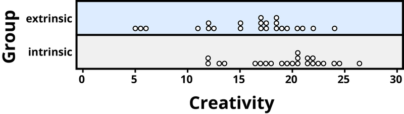
In this example, the key question is whether the type of motivation affects creativity scores. In particular, do subjects who were asked about intrinsic motivations tend to have higher creativity scores than subjects who were asked about extrinsic motivations?
Figure 2 reveals that both motivation groups saw considerable variability in creativity scores, and these scores have considerable overlap between the groups. In other words, it’s certainly not always the case that those with extrinsic motivations have higher creativity than those with intrinsic motivations, but there may still be a statistical tendency in this direction. (Psychologist Keith Stanovich (2013) refers to people’s difficulties with thinking about such probabilistic tendencies as “the Achilles heel of human cognition.”)
The mean creativity score is 19.88 for the intrinsic group, compared to 15.74 for the extrinsic group, which supports the researchers’ conjecture. Yet comparing only the means of the two groups fails to consider the variability of creativity scores in the groups. We can measure variability with statistics using, for instance, the standard deviation: 5.25 for the extrinsic group and 4.40 for the intrinsic group. The standard deviations tell us that most of the creativity scores are within about 5 points of the mean score in each group. We see that the mean score for the intrinsic group lies within one standard deviation of the mean score for extrinsic group. So, although there is a tendency for the creativity scores to be higher in the intrinsic group, on average, the difference is not extremely large.
We again want to consider possible explanations for this difference. The study only involved individuals with extensive creative writing experience. Although this limits the population to which we can generalize, it does not explain why the mean creativity score was a bit larger for the intrinsic group than for the extrinsic group. Maybe women tend to receive higher creativity scores? Here is where we need to focus on how the individuals were assigned to the motivation groups. If only women were in the intrinsic motivation group and only men in the extrinsic group, then this would present a problem because we wouldn’t know if the intrinsic group did better because of the different type of motivation or because they were women. However, the researchers guarded against such a problem by randomly assigning the individuals to the motivation groups. Like flipping a coin, each individual was just as likely to be assigned to either type of motivation. Why is this helpful? Because this random assignment tends to balance out all the variables related to creativity we can think of, and even those we don’t think of in advance, between the two groups. So we should have a similar male/female split between the two groups; we should have a similar age distribution between the two groups; we should have a similar distribution of educational background between the two groups; and so on. Random assignment should produce groups that are as similar as possible except for the type of motivation, which presumably eliminates all those other variables as possible explanations for the observed tendency for higher scores in the intrinsic group.
But does this always work? No, so by “luck of the draw” the groups may be a little different prior to answering the motivation survey. So then the question is, is it possible that an unlucky random assignment is responsible for the observed difference in creativity scores between the groups? In other words, suppose each individual’s poem was going to get the same creativity score no matter which group they were assigned to, that the type of motivation in no way impacted their score. Then how often would the random-assignment process alone lead to a difference in mean creativity scores as large (or larger) than 19.88 – 15.74 = 4.14 points?
We again want to apply to a probability model to approximate a p-value, but this time the model will be a bit different. Think of writing everyone’s creativity scores on an index card, shuffling up the index cards, and then dealing out 23 to the extrinsic motivation group and 24 to the intrinsic motivation group, and finding the difference in the group means. We (better yet, the computer) can repeat this process over and over to see how often, when the scores don’t change, random assignment leads to a difference in means at least as large as 4.41. Figure 3 shows the results from 1,000 such hypothetical random assignments for these scores.
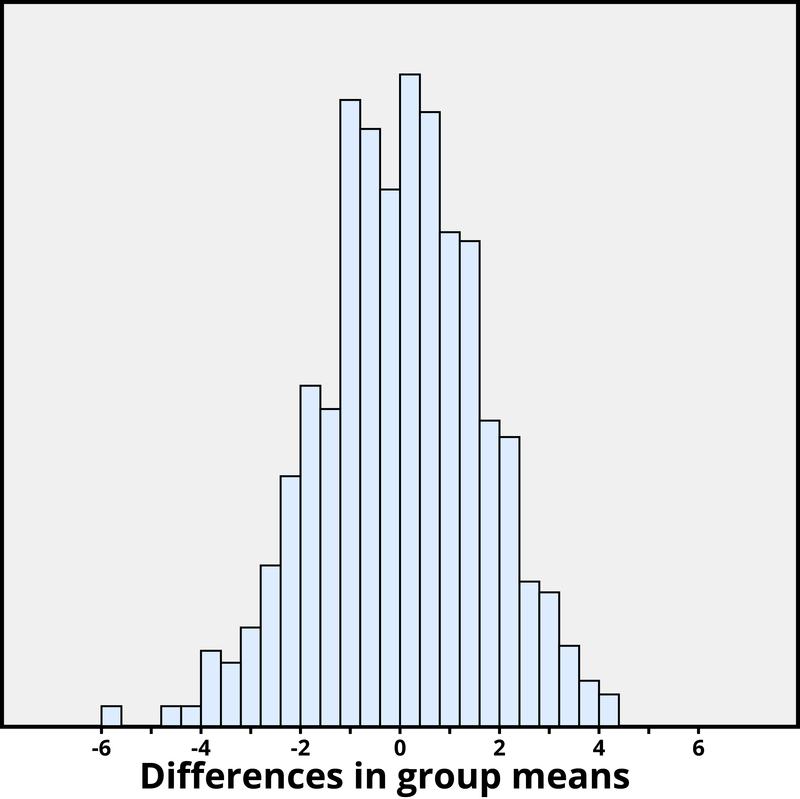
Only 2 of the 1,000 simulated random assignments produced a difference in group means of 4.41 or larger. In other words, the approximate p-value is 2/1000 = 0.002. This small p-value indicates that it would be very surprising for the random assignment process alone to produce such a large difference in group means. Therefore, as with Example 2, we have strong evidence that focusing on intrinsic motivations tends to increase creativity scores, as compared to thinking about extrinsic motivations.
Notice that the previous statement implies a cause-and-effect relationship between motivation and creativity score; is such a strong conclusion justified? Yes, because of the random assignment used in the study. That should have balanced out any other variables between the two groups, so now that the small p-value convinces us that the higher mean in the intrinsic group wasn’t just a coincidence, the only reasonable explanation left is the difference in the type of motivation. Can we generalize this conclusion to everyone? Not necessarily—we could cautiously generalize this conclusion to individuals with extensive experience in creative writing similar the individuals in this study, but we would still want to know more about how these individuals were selected to participate.
Conclusion

Statistical thinking involves the careful design of a study to collect meaningful data to answer a focused research question, detailed analysis of patterns in the data, and drawing conclusions that go beyond the observed data. Random sampling is paramount to generalizing results from our sample to a larger population, and random assignment is key to drawing cause-and-effect conclusions. With both kinds of randomness, probability models help us assess how much random variation we can expect in our results, in order to determine whether our results could happen by chance alone and to estimate a margin of error.
So where does this leave us with regard to the coffee study mentioned previously (the Freedman, Park, Abnet, Hollenbeck, & Sinha, 2012 found that men who drank at least six cups of coffee a day had a 10% lower chance of dying (women 15% lower) than those who drank none)? We can answer many of the questions:
- This was a 14-year study conducted by researchers at the National Cancer Institute.
- The results were published in the June issue of the New England Journal of Medicine, a respected, peer-reviewed journal.
- The study reviewed coffee habits of more than 402,000 people ages 50 to 71 from six states and two metropolitan areas. Those with cancer, heart disease, and stroke were excluded at the start of the study. Coffee consumption was assessed once at the start of the study.
- About 52,000 people died during the course of the study.
- People who drank between two and five cups of coffee daily showed a lower risk as well, but the amount of reduction increased for those drinking six or more cups.
- The sample sizes were fairly large and so the p-values are quite small, even though percent reduction in risk was not extremely large (dropping from a 12% chance to about 10%–11%).
- Whether coffee was caffeinated or decaffeinated did not appear to affect the results.
- This was an observational study, so no cause-and-effect conclusions can be drawn between coffee drinking and increased longevity, contrary to the impression conveyed by many news headlines about this study. In particular, it’s possible that those with chronic diseases don’t tend to drink coffee.
This study needs to be reviewed in the larger context of similar studies and consistency of results across studies, with the constant caution that this was not a randomized experiment. Whereas a statistical analysis can still “adjust” for other potential confounding variables, we are not yet convinced that researchers have identified them all or completely isolated why this decrease in death risk is evident. Researchers can now take the findings of this study and develop more focused studies that address new questions.
Learn More
Explore these outside resources to learn more about applied statistics:
- Video about p-values: P-Value Extravaganza
- Interactive web applets for teaching and learning statistics
- Inter-university Consortium for Political and Social Research where you can find and analyze data.
- The Consortium for the Advancement of Undergraduate Statistics
Think It Over
- Find a recent research article in your field and answer the following: What was the primary research question? How were individuals selected to participate in the study? Were summary results provided? How strong is the evidence presented in favor or against the research question? Was random assignment used? Summarize the main conclusions from the study, addressing the issues of statistical significance, statistical confidence, generalizability, and cause and effect. Do you agree with the conclusions drawn from this study, based on the study design and the results presented?
- Is it reasonable to use a random sample of 1,000 individuals to draw conclusions about all U.S. adults? Explain why or why not.
Licenses and Attributions (Click to expand)
CC licensed content, Original
- Modification, adaptation, and original content. Authored by: Pat Carroll and Lumen Learning. Provided by: Lumen Learning. License: CC BY: Attribution
CC licensed content, Shared previously
- Statistical Thinking. Authored by: Beth Chance and Allan Rossman, California Polytechnic State University, San Luis Obispo. Provided by: Noba. Located at: http://nobaproject.com/modules/statistical-thinking. License: CC BY-NC-SA: Attribution-NonCommercial-ShareAlike
- The Replication Crisis. Authored by: Colin Thomas William. Provided by: Ivy Tech Community College. License: CC BY: Attribution
related to whether the results from the sample can be generalized to a larger population.
the collection of individuals on which we collect data.
a larger collection of individuals that we would like to generalize our results to.
using a probability-based method to select a subset of individuals for the sample from the population.
the expected amount of random variation in a statistic; often defined for 95% confidence level.
using a probability-based method to divide a sample into treatment groups.
the probability of observing a particular outcome in a sample, or more extreme, under a conjecture about the larger population or process.
related to whether we say one variable is causing changes in the other variable, versus other variables that may be related to these two variables.
