
4 Motion in Two and Three Dimensions
4.2 Acceleration Vector
Learning Objectives
By the end of this section, you will be able to:
- Calculate the acceleration vector given the velocity function in unit vector notation.
- Describe the motion of a particle with a constant acceleration in three dimensions.
- Use the one-dimensional motion equations along perpendicular axes to solve a problem in two or three dimensions with a constant acceleration.
- Express the acceleration in unit vector notation.
Instantaneous Acceleration
In addition to obtaining the displacement and velocity vectors of an object in motion, we often want to know its acceleration vector at any point in time along its trajectory. This acceleration vector is the instantaneous acceleration and it can be obtained from the derivative with respect to time of the velocity function, as we have seen in a previous chapter. The only difference in two or three dimensions is that these are now vector quantities. Taking the derivative with respect to time [latex]\mathbf{\overset{\to }{v}}(t),[/latex] we find
The acceleration in terms of components is
Also, since the velocity is the derivative of the position function, we can write the acceleration in terms of the second derivative of the position function:
Example
Finding an Acceleration Vector
A particle has a velocity of [latex]\mathbf{\overset{\to }{v}}(t)=5.0t\mathbf{\hat{i}}+{t}^{2}\mathbf{\hat{j}}-2.0{t}^{3}\mathbf{\hat{k}}\text{m/s}.[/latex] (a) What is the acceleration function? (b) What is the acceleration vector at t = 2.0 s? Find its magnitude and direction.
Solution
Show Answer
(a) We take the first derivative with respect to time of the velocity function to find the acceleration. The derivative is taken component by component:
[latex]\mathbf{\overset{\to }{a}}(t)=5.0\mathbf{\hat{i}}+2.0t\mathbf{\hat{j}}-6.0{t}^{2}\mathbf{\hat{k}}\text{m/}{\text{s}}^{2}.[/latex] (b) Evaluating [latex]\mathbf{\overset{\to }{a}}(2.0\,\text{s})=5.0\mathbf{\hat{i}}+4.0\mathbf{\hat{j}}-24.0\mathbf{\hat{k}}\text{m/}{\text{s}}^{2}[/latex] gives us the direction in unit vector notation. The magnitude of the acceleration is [latex]|\mathbf{\overset{\to }{a}}(2.0\,\text{s})|=\sqrt{{5.0}^{2}+{4.0}^{2}+{(-24.0)}^{2}}=24.8\,\text{m/}{\text{s}}^{2}.[/latex]
Significance
In this example we find that acceleration has a time dependence and is changing throughout the motion. Let’s consider a different velocity function for the particle.
Example
Finding a Particle Acceleration
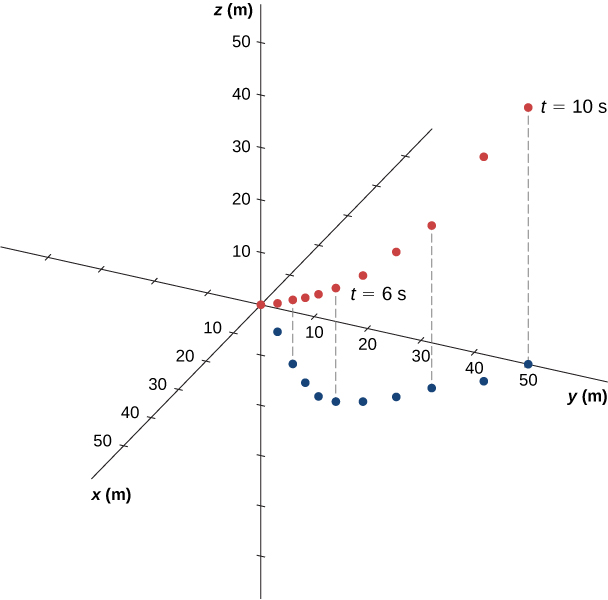
A particle has a position function [latex]\mathbf{\overset{\to }{r}}(t)=(10t-{t}^{2})\mathbf{\hat{i}}+5t\mathbf{\hat{j}}+5t\text{}\mathbf{\hat{k}}\text{m}.[/latex] (a) What is the velocity? (b) What is the acceleration? (c) Describe the motion from t = 0 s.
Strategy
We can gain some insight into the problem by looking at the position function. It is linear in y and z, so we know the acceleration in these directions is zero when we take the second derivative. Also, note that the position in the x direction is zero for t = 0 s and t = 10 s.
Solution
(a)
Show Answer
Taking the derivative with respect to time of the position function, we find [latex]\mathbf{\overset{\to }{v}}(t)=(10-2t)\mathbf{\hat{i}}+5\mathbf{\hat{j}}+5\mathbf{\hat{k}}\,\text{m/s}.[/latex] The velocity function is linear in time in the x direction and is constant in the y and z directions.
(b)
Show Answer
Taking the derivative of the velocity function, we find [latex]\mathbf{\overset{\to }{a}}(t)=-2\mathbf{\hat{i}}\,{\text{m/s}}^{2}.[/latex] The acceleration vector is a constant in the negative x-direction.
(c)
Show Answer
The trajectory of the particle can be seen in Figure.
Let’s look in the y and z directions first. The particle’s position increases steadily as a function of time with a constant velocity in these directions. In the x direction, however, the particle follows a path in positive x until t = 5 s, when it reverses direction. We know this from looking at the velocity function, which becomes zero at this time and negative thereafter. We also know this because the acceleration is negative and constant—meaning, the particle is decelerating, or accelerating in the negative direction. The particle’s position reaches 25 m, where it then reverses direction and begins to accelerate in the negative x direction. The position reaches zero at t = 10 s.
Significance
By graphing the trajectory of the particle, we can better understand its motion, given by the numerical results of the kinematic equations.
Check Your Understanding
Suppose the acceleration function has the form [latex]\mathbf{\overset{\to }{a}}(t)=a\mathbf{\hat{i}}+b\mathbf{\hat{j}}+c\mathbf{\hat{k}}\text{m/}{\text{s}}^{2},[/latex] where a, b, and c are constants. What can be said about the functional form of the velocity function?
Show Solution
The acceleration vector is constant and doesn’t change with time. If a, b, and c are not zero, then the velocity function must be linear in time. We have [latex]\mathbf{\overset{\to }{v}}(t)=\int \mathbf{\overset{\to }{a}}dt=\int (a\mathbf{\hat{i}}+b\mathbf{\hat{j}}+c\mathbf{\hat{k}})dt=(a\mathbf{\hat{i}}+b\mathbf{\hat{j}}+c\mathbf{\hat{k}})t\,\text{m/s},[/latex] since taking the derivative of the velocity function produces [latex]\mathbf{\overset{\to }{a}}(t).[/latex] If any of the components of the acceleration are zero, then that component of the velocity would be a constant.
Constant Acceleration
Multidimensional motion with constant acceleration can be treated the same way as shown in the previous chapter for one-dimensional motion. Earlier we showed that three-dimensional motion is equivalent to three one-dimensional motions, each along an axis perpendicular to the others. To develop the relevant equations in each direction, let’s consider the two-dimensional problem of a particle moving in the xy plane with constant acceleration, ignoring the z-component for the moment. The acceleration vector is
Each component of the motion has a separate set of equations similar to Figure–Figure of the previous chapter on one-dimensional motion. We show only the equations for position and velocity in the x– and y-directions. A similar set of kinematic equations could be written for motion in the z-direction:
Here the subscript 0 denotes the initial position or velocity. Figure to Figure can be substituted into Figure and Figure without the z-component to obtain the position vector and velocity vector as a function of time in two dimensions:
The following example illustrates a practical use of the kinematic equations in two dimensions.
Example
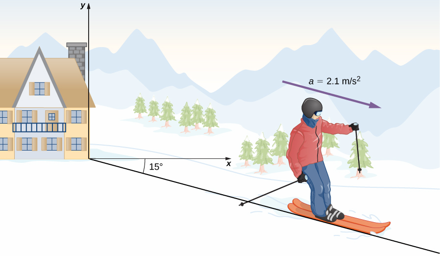
A SkierFigure shows a skier moving with an acceleration of [latex]2.1\,\text{m/}{\text{s}}^{2}[/latex] down a slope of [latex]15^\circ[/latex] at t = 0. With the origin of the coordinate system at the front of the lodge, her initial position and velocity are
and
(a) What are the x- and y-components of the skier’s position and velocity as functions of time? (b) What are her position and velocity at t = 10.0 s?
Strategy
Since we are evaluating the components of the motion equations in the x and y directions, we need to find the components of the acceleration and put them into the kinematic equations. The components of the acceleration are found by referring to the coordinate system in Figure. Then, by inserting the components of the initial position and velocity into the motion equations, we can solve for her position and velocity at a later time t.
Solution
Show Answer
(a)
The origin of the coordinate system is at the top of the hill with y-axis vertically upward and the x-axis horizontal. By looking at the trajectory of the skier, the x-component of the acceleration is positive and the y-component is negative. Since the angle is [latex]15^\circ[/latex] down the slope, we find
[latex]{a}_{x}=(2.1\,\text{m/}{\text{s}}^{2})\,\text{cos}(15^\circ)=2.0\,\text{m/}{\text{s}}^{2}[/latex] [latex]{a}_{y}=(-2.1\,\text{m/}{\text{s}}^{2})\,\text{sin}\,15^\circ=-0.54\,\text{m/}{\text{s}}^{2}.[/latex]
Inserting the initial position and velocity into (Figure) and (Figure) for x, we have
[latex]x(t)=75.0\,\text{m}+(4.1\,\text{m/s})t+\frac{1}{2}(2.0\,\text{m/}{\text{s}}^{2}){t}^{2}[/latex] [latex]{v}_{x}(t)=4.1\,\text{m/s}+(2.0\,\text{m/}{\text{s}}^{2})t.[/latex]
For y, we have
[latex]y(t)=-50.0\,\text{m}+(-1.1\,\text{m/s})t+\frac{1}{2}(-0.54\,\text{m/}{\text{s}}^{2}){t}^{2}[/latex] [latex]{v}_{y}(t)=-1.1\,\text{m/s}+(-0.54\,\text{m/}{\text{s}}^{2})t.[/latex]
(b) Now that we have the equations of motion for x and y as functions of time, we can evaluate them at t = 10.0 s:
[latex]x(10.0\,\text{s})=75.0\,\text{m}+(4.1\,\text{m/}{\text{s}}^{2})(10.0\,\text{s})+\frac{1}{2}(2.0\,\text{m/}{\text{s}}^{2}){(10.0\,\text{s})}^{2}=216.0\,\text{m}[/latex] [latex]{v}_{x}(10.0\,\text{s})=4.1\,\text{m/s}+(2.0\,\text{m/}{\text{s}}^{2})(10.0\,\text{s})=24.1\text{m}\text{/s}[/latex] [latex]y(10.0\,\text{s})=-50.0\,\text{m}+(-1.1\,\text{m/s})(10.0\,\text{s})+\frac{1}{2}(-0.54\,\text{m/}{\text{s}}^{2}){(10.0\,\text{s})}^{2}=-88.0\,\text{m}[/latex] [latex]{v}_{y}(10.0\,\text{s})=-1.1\,\text{m/s}+(-0.54\,\text{m/}{\text{s}}^{2})(10.0\,\text{s})=-6.5\,\text{m/s}.[/latex]
The position and velocity at t = 10.0 s are, finally,
[latex]\mathbf{\overset{\to }{r}}(10.0\,\text{s})=(216.0\mathbf{\hat{i}}-88.0\mathbf{\hat{j}})\,\text{m}[/latex] [latex]\mathbf{\overset{\to }{v}}(10.0\,\text{s})=(24.1\mathbf{\hat{i}}-6.5\mathbf{\hat{j}})\text{m/s}.[/latex]
The magnitude of the velocity of the skier at 10.0 s is 25 m/s, which is 60 mi/h.
Significance
It is useful to know that, given the initial conditions of position, velocity, and acceleration of an object, we can find the position, velocity, and acceleration at any later time.
With Figure through Figure we have completed the set of expressions for the position, velocity, and acceleration of an object moving in two or three dimensions. If the trajectories of the objects look something like the “Red Arrows” in the opening picture for the chapter, then the expressions for the position, velocity, and acceleration can be quite complicated. In the sections to follow we examine two special cases of motion in two and three dimensions by looking at projectile motion and circular motion.
At this University of Colorado Boulder website, you can explore the position velocity and acceleration of a ladybug with an interactive simulation that allows you to change these parameters.
Summary
- In two and three dimensions, the acceleration vector can have an arbitrary direction and does not necessarily point along a given component of the velocity.
- The instantaneous acceleration is produced by a change in velocity taken over a very short (infinitesimal) time period. Instantaneous acceleration is a vector in two or three dimensions. It is found by taking the derivative of the velocity function with respect to time.
- In three dimensions, acceleration [latex]\mathbf{\overset{\to }{a}}(t)[/latex] can be written as a vector sum of the one-dimensional accelerations [latex]{a}_{x}(t),{a}_{y}(t),\text{and}\,{a}_{z}(t)[/latex] along the x-, y-, and z-axes.
- The kinematic equations for constant acceleration can be written as the vector sum of the constant acceleration equations in the x, y, and z directions.
Conceptual Questions
If the position function of a particle is a linear function of time, what can be said about its acceleration?
If an object has a constant x-component of the velocity and suddenly experiences an acceleration in the y direction, does the x-component of its velocity change?
Show Solution
No, motions in perpendicular directions are independent.
If an object has a constant x-component of velocity and suddenly experiences an acceleration at an angle of [latex]70^\circ[/latex] in the x direction, does the x-component of velocity change?
Problems
The position of a particle is [latex]\mathbf{\overset{\to }{r}}(t)=(3.0{t}^{2}\mathbf{\hat{i}}+5.0\mathbf{\hat{j}}-6.0t\mathbf{\hat{k}})\,\text{m}.[/latex] (a) Determine its velocity and acceleration as functions of time. (b) What are its velocity and acceleration at time t = 0?
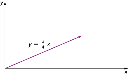
A particle’s acceleration is [latex](4.0\mathbf{\hat{i}}+3.0\mathbf{\hat{j}})\text{m/}{\text{s}}^{2}.[/latex] At t = 0, its position and velocity are zero. (a) What are the particle’s position and velocity as functions of time? (b) Find the equation of the path of the particle. Draw the x- and y-axes and sketch the trajectory of the particle.
Show Solution
a. [latex]\mathbf{\overset{\to }{v}}(t)=(4.0t\mathbf{\hat{i}}+3.0t\mathbf{\hat{j}})\text{m/s},[/latex] [latex]\mathbf{\overset{\to }{r}}(t)=(2.0{t}^{2}\mathbf{\hat{i}}+\frac{3}{2}{t}^{2}\mathbf{\hat{j}})\,\text{m}[/latex],
b. [latex]x(t)=2.0{t}^{2}\text{m,}\,y(t)=\frac{3}{2}{t}^{2}\text{m,}\,{t}^{2}=\frac{x}{2}\Rightarrow y=\frac{3}{4}x[/latex]
A boat leaves the dock at t = 0 and heads out into a lake with an acceleration of [latex]2.0\,\text{m/}{\text{s}}^{2}\mathbf{\hat{i}}.[/latex] A strong wind is pushing the boat, giving it an additional velocity of [latex]2.0\,\text{m/s}\mathbf{\hat{i}}+1.0\,\text{m/s}\mathbf{\hat{j}}.[/latex] (a) What is the velocity of the boat at t = 10 s? (b) What is the position of the boat at t = 10s? Draw a sketch of the boat’s trajectory and position at t = 10 s, showing the x- and y-axes.
The position of a particle for t > 0 is given by [latex]\mathbf{\overset{\to }{r}}(t)=(3.0{t}^{2}\mathbf{\hat{i}}-7.0{t}^{3}\mathbf{\hat{j}}-5.0{t}^{-2}\mathbf{\hat{k}})\,\text{m}.[/latex] (a) What is the velocity as a function of time? (b) What is the acceleration as a function of time? (c) What is the particle’s velocity at t = 2.0 s? (d) What is its speed at t = 1.0 s and t = 3.0 s? (e) What is the average velocity between t = 1.0 s and t = 2.0 s?
Show Solution
a. [latex]\mathbf{\overset{\to }{v}}(t)=(6.0t\mathbf{\hat{i}}-21.0{t}^{2}\mathbf{\hat{j}}+10.0{t}^{-3}\mathbf{\hat{k}})\text{m/s}[/latex],
b. [latex]\mathbf{\overset{\to }{a}}(t)=(6.0\mathbf{\hat{i}}-42.0t\mathbf{\hat{j}}-30{t}^{-4}\mathbf{\hat{k}})\text{m/}{\text{s}}^{2}[/latex],
c. [latex]\mathbf{\overset{\to }{v}}(2.0s)=(12.0\mathbf{\hat{i}}-84.0\mathbf{\hat{j}}+1.25\mathbf{\hat{k}})\text{m/s}[/latex],
d. [latex]\mathbf{\overset{\to }{v}}(1.0\,\text{s})=6.0\mathbf{\hat{i}}-21.0\mathbf{\hat{j}}+10.0\mathbf{\hat{k}}\text{m/s},\,|\mathbf{\overset{\to }{v}}(1.0\,\text{s})|=24.0\,\text{m/s}[/latex]
[latex]\mathbf{\overset{\to }{v}}(3.0\,\text{s})=18.0\mathbf{\hat{i}}-189.0\mathbf{\hat{j}}+0.37\mathbf{\hat{k}}\text{m/s},[/latex] [latex]|\mathbf{\overset{\to }{v}}(3.0\,\text{s})|=199.0\,\text{m/s}[/latex],
e. [latex]\mathbf{\overset{\to }{r}}(t)=(3.0{t}^{2}\mathbf{\hat{i}}-7.0{t}^{3}\mathbf{\hat{j}}-5.0{t}^{-2}\mathbf{\hat{k}})\text{cm}[/latex]
[latex]\begin{array}{cc} \hfill {\mathbf{\overset{\to }{v}}}_{\text{avg}}& =9.0\mathbf{\hat{i}}-49.0\mathbf{\hat{j}}-6.3\mathbf{\hat{k}}\text{m/s}\hfill \end{array}[/latex]
The acceleration of a particle is a constant. At t = 0 the velocity of the particle is [latex](10\mathbf{\hat{i}}+20\mathbf{\hat{j}})\text{m/s}.[/latex] At t = 4 s the velocity is [latex]10\mathbf{\hat{j}}\text{m/s}.[/latex] (a) What is the particle’s acceleration? (b) How do the position and velocity vary with time? Assume the particle is initially at the origin.
A particle has a position function [latex]\mathbf{\overset{\to }{r}}(t)=\text{cos}(1.0t)\mathbf{\hat{i}}+\text{sin}(1.0t)\mathbf{\hat{j}}+t\mathbf{\hat{k}},[/latex] where the arguments of the cosine and sine functions are in radians. (a) What is the velocity vector? (b) What is the acceleration vector?
Show Solution
a. [latex]\mathbf{\overset{\to }{v}}(t)=\text{−sin}(1.0t)\mathbf{\hat{i}}+\text{cos}(1.0t)\mathbf{\hat{j}}+\mathbf{\hat{k}}[/latex], b. [latex]\mathbf{\overset{\to }{a}}(t)=\text{−cos}(1.0t)\mathbf{\hat{i}}-\text{sin}(1.0t)\mathbf{\hat{j}}[/latex]
A Lockheed Martin F-35 II Lighting jet takes off from an aircraft carrier with a runway length of 90 m and a takeoff speed 70 m/s at the end of the runway. Jets are catapulted into airspace from the deck of an aircraft carrier with two sources of propulsion: the jet propulsion and the catapult. At the point of leaving the deck of the aircraft carrier, the F-35’s acceleration decreases to a constant acceleration of [latex]5.0\,\text{m/}{\text{s}}^{2}[/latex] at [latex]30^\circ[/latex] with respect to the horizontal. (a) What is the initial acceleration of the F-35 on the deck of the aircraft carrier to make it airborne? (b) Write the position and velocity of the F-35 in unit vector notation from the point it leaves the deck of the aircraft carrier. (c) At what altitude is the fighter 5.0 s after it leaves the deck of the aircraft carrier? (d) What is its velocity and speed at this time? (e) How far has it traveled horizontally?
Glossary
- acceleration vector
- instantaneous acceleration found by taking the derivative of the velocity function with respect to time in unit vector notation