15.5 Damped Oscillations

In the real world, oscillations seldom follow true SHM. Friction of some sort usually acts to dampen the motion so it dies away, or needs more force to continue. In this section, we examine some examples of damped harmonic motion and see how to modify the equations of motion to describe this more general case.

A guitar string stops oscillating a few seconds after being plucked. To keep swinging on a playground swing, you must keep pushing (Figure). Although we can often make friction and other nonconservative forces small or negligible, completely undamped motion is rare. In fact, we may even want to damp oscillations, such as with car shock absorbers.

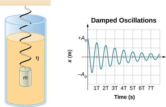
Figure shows a mass m attached to a spring with a force constant [latex]k.[/latex] The mass is raised to a position [latex]{A}_{0}[/latex], the initial amplitude, and then released. The mass oscillates around the equilibrium position in a fluid with viscosity but the amplitude decreases for each oscillation. For a system that has a small amount of damping, the period and frequency are constant and are nearly the same as for SHM, but the amplitude gradually decreases as shown. This occurs because the non-conservative damping force removes energy from the system, usually in the form of thermal energy.

Consider the forces acting on the mass. Note that the only contribution of the weight is to change the equilibrium position, as discussed earlier in the chapter. Therefore, the net force is equal to the force of the spring and the damping force [latex]({F}_{D})[/latex]. If the magnitude of the velocity is small, meaning the mass oscillates slowly, the damping force is proportional to the velocity and acts against the direction of motion [latex]({F}_{D}=\text{−}bv)[/latex]. The net force on the mass is therefore

Writing this as a differential equation in x, we obtain

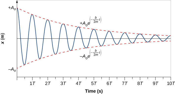
To determine the solution to this equation, consider the plot of position versus time shown in Figure. The curve resembles a cosine curve oscillating in the envelope of an exponential function [latex]{A}_{0}{e}^{\text{−}\alpha t}[/latex] where [latex]\alpha =\frac{b}{2m}[/latex]. The solution is

It is left as an exercise to prove that this is, in fact, the solution. To prove that it is the right solution, take the first and second derivatives with respect to time and substitute them into Figure. It is found that Figure is the solution if

Recall that the angular frequency of a mass undergoing SHM is equal to the square root of the force constant divided by the mass. This is often referred to as the natural angular frequency, which is represented as

The angular frequency for damped harmonic motion becomes

Recall that when we began this description of damped harmonic motion, we stated that the damping must be small. Two questions come to mind. Why must the damping be small? And how small is small? If you gradually increase the amount of damping in a system, the period and frequency begin to be affected, because damping opposes and hence slows the back and forth motion. (The net force is smaller in both directions.) If there is very large damping, the system does not even oscillate—it slowly moves toward equilibrium. The angular frequency is equal to

As b increases, [latex]\frac{k}{m}-{(\frac{b}{2m})}^{2}[/latex] becomes smaller and eventually reaches zero when [latex]b=\sqrt{4mk}[/latex]. If b becomes any larger, [latex]\frac{k}{m}-{(\frac{b}{2m})}^{2}[/latex] becomes a negative number and [latex]\sqrt{\frac{k}{m}-{(\frac{b}{2m})}^{2}}[/latex] is a complex number.

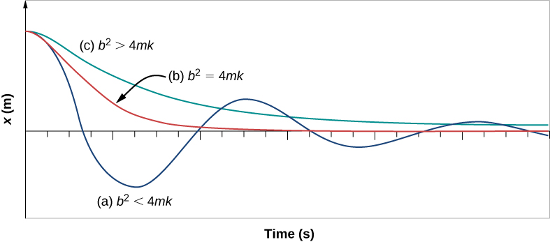
Figure shows the displacement of a harmonic oscillator for different amounts of damping. When the damping constant is small, [latex]b \lt \sqrt{4mk}[/latex], the system oscillates while the amplitude of the motion decays exponentially. This system is said to be underdamped, as in curve (a). Many systems are underdamped, and oscillate while the amplitude decreases exponentially, such as the mass oscillating on a spring. The damping may be quite small, but eventually the mass comes to rest. If the damping constant is [latex]b=\sqrt{4mk}[/latex], the system is said to be critically damped, as in curve (b). An example of a critically damped system is the shock absorbers in a car. It is advantageous to have the oscillations decay as fast as possible. Here, the system does not oscillate, but asymptotically approaches the equilibrium condition as quickly as possible. Curve (c) in Figure represents an overdamped system where [latex]b \gt \sqrt{4mk}.[/latex] An overdamped system will approach equilibrium over a longer period of time.

Critical damping is often desired, because such a system returns to equilibrium rapidly and remains at equilibrium as well. In addition, a constant force applied to a critically damped system moves the system to a new equilibrium position in the shortest time possible without overshooting or oscillating about the new position.