
10 Fixed-Axis Rotation
10.2 Rotation with Constant Angular Acceleration
Learning Objectives
By the end of this section, you will be able to:
- Derive the kinematic equations for rotational motion with constant angular acceleration
- Select from the kinematic equations for rotational motion with constant angular acceleration the appropriate equations to solve for unknowns in the analysis of systems undergoing fixed-axis rotation
- Use solutions found with the kinematic equations to verify the graphical analysis of fixed-axis rotation with constant angular acceleration
In the preceding section, we defined the rotational variables of angular displacement, angular velocity, and angular acceleration. In this section, we work with these definitions to derive relationships among these variables and use these relationships to analyze rotational motion for a rigid body about a fixed axis under a constant angular acceleration. This analysis forms the basis for rotational kinematics. If the angular acceleration is constant, the equations of rotational kinematics simplify, similar to the equations of linear kinematics discussed in Motion along a Straight Line and Motion in Two and Three Dimensions. We can then use this simplified set of equations to describe many applications in physics and engineering where the angular acceleration of the system is constant. Rotational kinematics is also a prerequisite to the discussion of rotational dynamics later in this chapter.
Kinematics of Rotational Motion
Using our intuition, we can begin to see how the rotational quantities [latex]\theta ,[/latex] [latex]\omega ,[/latex] [latex]\alpha[/latex], and t are related to one another. For example, we saw in the preceding section that if a flywheel has an angular acceleration in the same direction as its angular velocity vector, its angular velocity increases with time and its angular displacement also increases. On the contrary, if the angular acceleration is opposite to the angular velocity vector, its angular velocity decreases with time. We can describe these physical situations and many others with a consistent set of rotational kinematic equations under a constant angular acceleration. The method to investigate rotational motion in this way is called kinematics of rotational motion.
To begin, we note that if the system is rotating under a constant acceleration, then the average angular velocity follows a simple relation because the angular velocity is increasing linearly with time. The average angular velocity is just half the sum of the initial and final values:
From the definition of the average angular velocity, we can find an equation that relates the angular position, average angular velocity, and time:
Solving for [latex]\theta[/latex], we have
where we have set [latex]{t}_{0}=0[/latex]. This equation can be very useful if we know the average angular velocity of the system. Then we could find the angular displacement over a given time period. Next, we find an equation relating [latex]\omega[/latex], [latex]\alpha[/latex], and t. To determine this equation, we start with the definition of angular acceleration:
We rearrange this to get [latex]\alpha dt=d\omega[/latex] and then we integrate both sides of this equation from initial values to final values, that is, from [latex]{t}_{0}[/latex] to t and [latex]{\omega }_{0}\,\text{to}\,{\omega }_{\text{f}}[/latex]. In uniform rotational motion, the angular acceleration is constant so it can be pulled out of the integral, yielding two definite integrals:
Setting [latex]{t}_{0}=0[/latex], we have
We rearrange this to obtain
where [latex]{\omega }_{0}[/latex] is the initial angular velocity. Figure is the rotational counterpart to the linear kinematics equation [latex]{v}_{\text{f}}={v}_{0}+at[/latex]. With Figure, we can find the angular velocity of an object at any specified time t given the initial angular velocity and the angular acceleration.
Let’s now do a similar treatment starting with the equation [latex]\omega =\frac{d\theta }{dt}[/latex]. We rearrange it to obtain [latex]\omega dt=d\theta[/latex] and integrate both sides from initial to final values again, noting that the angular acceleration is constant and does not have a time dependence. However, this time, the angular velocity is not constant (in general), so we substitute in what we derived above:
where we have set [latex]{t}_{0}=0[/latex]. Now we rearrange to obtain
Figure is the rotational counterpart to the linear kinematics equation found in Motion Along a Straight Line for position as a function of time. This equation gives us the angular position of a rotating rigid body at any time t given the initial conditions (initial angular position and initial angular velocity) and the angular acceleration.
We can find an equation that is independent of time by solving for t in Figure and substituting into Figure. Figure becomes
or
Figure through Figure describe fixed-axis rotation for constant acceleration and are summarized in Figure.
| Angular displacement from average angular velocity | [latex]{\theta }_{\text{f}}={\theta }_{0}+\overset{–}{\omega }t[/latex] |
| Angular velocity from angular acceleration | [latex]{\omega }_{\text{f}}={\omega }_{0}+\alpha t[/latex] |
| Angular displacement from angular velocity and angular acceleration | [latex]{\theta }_{\text{f}}={\theta }_{0}+{\omega }_{0}t+\frac{1}{2}\alpha {t}^{2}[/latex] |
| Angular velocity from angular displacement and angular acceleration | [latex]{\omega }_{\text{f}}^{2}={\omega }_{0}{}^{2}+2\alpha (\Delta \theta )[/latex] |
Applying the Equations for Rotational Motion
Now we can apply the key kinematic relations for rotational motion to some simple examples to get a feel for how the equations can be applied to everyday situations.
Example
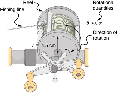
Calculating the Acceleration of a Fishing Reel
A deep-sea fisherman hooks a big fish that swims away from the boat, pulling the fishing line from his fishing reel. The whole system is initially at rest, and the fishing line unwinds from the reel at a radius of 4.50 cm from its axis of rotation. The reel is given an angular acceleration of [latex]110{\,\text{rad/s}}^{2}[/latex] for 2.00 s (Figure).
(a) What is the final angular velocity of the reel after 2 s?
(b) How many revolutions does the reel make?
Strategy
Identify the knowns and compare with the kinematic equations for constant acceleration. Look for the appropriate equation that can be solved for the unknown, using the knowns given in the problem description.
Solution
- We are given [latex]\alpha[/latex] and t and want to determine [latex]\omega[/latex]. The most straightforward equation to use is [latex]{\omega }_{\text{f}}={\omega }_{0}+\alpha t[/latex], since all terms are known besides the unknown variable we are looking for. We are given that [latex]{\omega }_{0}=0[/latex] (it starts from rest), so
[latex]{\omega }_{\text{f}}=0+(110{\,\text{rad/s}}^{2})(2.00\,\text{s})=220\,\text{rad/s}.[/latex]
- We are asked to find the number of revolutions. Because [latex]1\,\text{rev}=2\pi \,\text{rad}[/latex], we can find the number of revolutions by finding [latex]\theta[/latex] in radians. We are given [latex]\alpha[/latex] and t, and we know [latex]{\omega }_{0}[/latex] is zero, so we can obtain [latex]\theta[/latex] by using
[latex]\begin{array}{cc}\hfill {\theta }_{\text{f}}& ={\theta }_{\text{i}}+{\omega }_{\text{i}}t+\frac{1}{2}\alpha {t}^{2}\hfill \\ & =0+0+(0.500)(110{\,\text{rad/s}}^{2}){(2.00\,\text{s})}^{2}=220\,\text{rad}\text{.}\hfill \end{array}[/latex]
Converting radians to revolutions gives
[latex]\text{Number of rev}\,=(220\,\text{rad})\frac{1\,\text{rev}}{2\pi \,\text{rad}}=35.0\,\text{rev}\text{.}[/latex]
Significance
This example illustrates that relationships among rotational quantities are highly analogous to those among linear quantities. The answers to the questions are realistic. After unwinding for two seconds, the reel is found to spin at 220 rad/s, which is 2100 rpm. (No wonder reels sometimes make high-pitched sounds.)
In the preceding example, we considered a fishing reel with a positive angular acceleration. Now let us consider what happens with a negative angular acceleration.
Example
Calculating the Duration When the Fishing Reel Slows Down and Stops
Now the fisherman applies a brake to the spinning reel, achieving an angular acceleration of [latex]-300{\,\text{rad/s}}^{2}[/latex]. How long does it take the reel to come to a stop?
Strategy
We are asked to find the time t for the reel to come to a stop. The initial and final conditions are different from those in the previous problem, which involved the same fishing reel. Now we see that the initial angular velocity is [latex]{\omega }_{0}=220\,\text{rad}\text{/}\text{s}[/latex] and the final angular velocity [latex]\omega[/latex] is zero. The angular acceleration is given as [latex]\alpha =-300\,{\text{rad/s}}^{2}.[/latex] Examining the available equations, we see all quantities but t are known in [latex]{\omega }_{\text{f}}={\omega }_{0}+\alpha t[/latex], making it easiest to use this equation.
Solution
The equation states
We solve the equation algebraically for t and then substitute the known values as usual, yielding
Significance
Note that care must be taken with the signs that indicate the directions of various quantities. Also, note that the time to stop the reel is fairly small because the acceleration is rather large. Fishing lines sometimes snap because of the accelerations involved, and fishermen often let the fish swim for a while before applying brakes on the reel. A tired fish is slower, requiring a smaller acceleration.
Check Your Understanding
A centrifuge used in DNA extraction spins at a maximum rate of 7000 rpm, producing a “g-force” on the sample that is 6000 times the force of gravity. If the centrifuge takes 10 seconds to come to rest from the maximum spin rate: (a) What is the angular acceleration of the centrifuge? (b) What is the angular displacement of the centrifuge during this time?
Show Solution
a. Using Figure, we have [latex]7000\,\text{rpm}=\frac{7000.0(2\pi \,\text{rad})}{60.0\,\text{s}}=733.0\,\text{rad}\text{/}\text{s},[/latex]
[latex]\alpha =\frac{\omega -{\omega }_{0}}{t}=\frac{733.0\,\text{rad}\text{/}\text{s}}{10.0\,\text{s}}=73.3\,\text{rad}\text{/}{\text{s}}^{2}[/latex];
b. Using Figure, we have
[latex]{\omega }^{2}={\omega }_{0}^{2}+2\alpha \Delta \theta \Rightarrow \Delta \theta =\frac{{\omega }^{2}-{\omega }_{0}^{2}}{2\alpha }=\frac{0-{(733.0\,\text{rad}\text{/}\text{s})}^{2}}{2(73.3\,\text{rad}\text{/}{\text{s}}^{2})}=3665.2\,\text{rad}[/latex]
Example
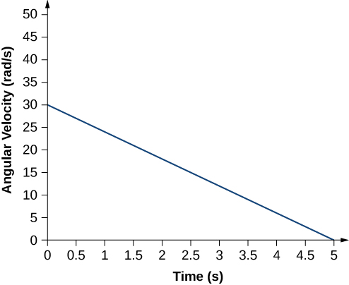
Angular Acceleration of a PropellerFigure shows a graph of the angular velocity of a propeller on an aircraft as a function of time. Its angular velocity starts at 30 rad/s and drops linearly to 0 rad/s over the course of 5 seconds. (a) Find the angular acceleration of the object and verify the result using the kinematic equations. (b) Find the angle through which the propeller rotates during these 5 seconds and verify your result using the kinematic equations.
Strategy
- Since the angular velocity varies linearly with time, we know that the angular acceleration is constant and does not depend on the time variable. The angular acceleration is the slope of the angular velocity vs. time graph, [latex]\alpha =\frac{d\omega }{dt}[/latex]. To calculate the slope, we read directly from Figure, and see that [latex]{\omega }_{0}=30\,\text{rad/s}[/latex] at [latex]t=0\,\text{s}[/latex] and [latex]{\omega }_{\text{f}}=0\,\text{rad/s}[/latex] at [latex]t=5\,\text{s}[/latex]. Then, we can verify the result using [latex]\omega ={\omega }_{0}+\alpha t[/latex].
- We use the equation [latex]\omega =\frac{d\theta }{dt};[/latex] since the time derivative of the angle is the angular velocity, we can find the angular displacement by integrating the angular velocity, which from the figure means taking the area under the angular velocity graph. In other words:
[latex]\underset{{\theta }_{0}}{\overset{{\theta }_{\text{f}}}{\int }}d\theta ={\theta }_{\text{f}}-{\theta }_{0}=\underset{{t}_{0}}{\overset{{t}_{\text{f}}}{\int }}\omega (t)dt.[/latex]
Then we use the kinematic equations for constant acceleration to verify the result.
Solution
- Calculating the slope, we get
[latex]\alpha =\frac{\omega -{\omega }_{0}}{t-{t}_{0}}=\frac{(0-30.0)\,\text{rad/s}}{(5.0-0)\,\text{s}}=-6.0\,{\text{rad/s}}^{2}.[/latex]
We see that this is exactly Figure with a little rearranging of terms.
- We can find the area under the curve by calculating the area of the right triangle, as shown in Figure.
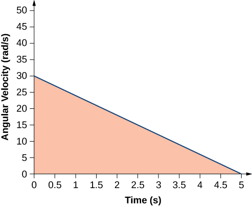
Figure 10.13 The area under the curve is the area of the right triangle. [latex]\begin{array}{ccc}\hfill \Delta \theta & =\hfill & \text{area}(\text{triangle});\hfill \\ \hfill \Delta \theta & =\hfill & \frac{1}{2}(30\,\text{rad/s})(5\,\text{s})=75\,\text{rad}\text{.}\hfill \end{array}[/latex]We verify the solution using Figure:
[latex]{\theta }_{\text{f}}={\theta }_{0}+{\omega }_{0}t+\frac{1}{2}\alpha {t}^{2}.[/latex]Setting [latex]{\theta }_{0}=0[/latex], we have
[latex]{\theta }_{0}=(30.0\,\text{rad}\text{/}\text{s})(5.0\,\text{s})+\frac{1}{2}{(-6.0\,\text{rad}\text{/}{\text{s}}^{2})(5.0\,\text{rad}\text{/}\text{s})}^{2}=150.0-75.0=75.0\,\text{rad}.[/latex]This verifies the solution found from finding the area under the curve.
Significance
We see from part (b) that there are alternative approaches to analyzing fixed-axis rotation with constant acceleration. We started with a graphical approach and verified the solution using the rotational kinematic equations. Since [latex]\alpha =\frac{d\omega }{dt}[/latex], we could do the same graphical analysis on an angular acceleration-vs.-time curve. The area under an [latex]\alpha \text{-vs.-}t[/latex] curve gives us the change in angular velocity. Since the angular acceleration is constant in this section, this is a straightforward exercise.
Summary
- The kinematics of rotational motion describes the relationships among rotation angle (angular position), angular velocity, angular acceleration, and time.
- For a constant angular acceleration, the angular velocity varies linearly. Therefore, the average angular velocity is 1/2 the initial plus final angular velocity over a given time period:
[latex]\overset{–}{\omega }=\frac{{\omega }_{0}+{\omega }_{\text{f}}}{2}.[/latex]
- We used a graphical analysis to find solutions to fixed-axis rotation with constant angular acceleration. From the relation [latex]\omega =\frac{d\theta }{dt}[/latex], we found that the area under an angular velocity-vs.-time curve gives the angular displacement, [latex]{\theta }_{\text{f}}-{\theta }_{0}=\Delta \theta =\underset{{t}_{0}}{\overset{t}{\int }}\omega (t)dt[/latex]. The results of the graphical analysis were verified using the kinematic equations for constant angular acceleration. Similarly, since [latex]\alpha =\frac{d\omega }{dt}[/latex], the area under an angular acceleration-vs.-time graph gives the change in angular velocity: [latex]{\omega }_{f}-{\omega }_{0}=\Delta \omega =\underset{{t}_{0}}{\overset{t}{\int }}\alpha (t)dt[/latex].
Conceptual Questions
If a rigid body has a constant angular acceleration, what is the functional form of the angular velocity in terms of the time variable?
Show Solution
straight line, linear in time variable
If a rigid body has a constant angular acceleration, what is the functional form of the angular position?
If the angular acceleration of a rigid body is zero, what is the functional form of the angular velocity?
Show Solution
constant
A massless tether with a masses tied to both ends rotates about a fixed axis through the center. Can the total acceleration of the tether/mass combination be zero if the angular velocity is constant?
Problems
A wheel has a constant angular acceleration of [latex]5.0\,\text{rad}\text{/}{\text{s}}^{2}[/latex]. Starting from rest, it turns through 300 rad. (a) What is its final angular velocity? (b) How much time elapses while it turns through the 300 radians?
Show Solution
a. [latex]\omega =54.8\,\text{rad}\text{/}\text{s}[/latex];
b. [latex]t=11.0\,\text{s}[/latex]
During a 6.0-s time interval, a flywheel with a constant angular acceleration turns through 500 radians that acquire an angular velocity of 100 rad/s. (a) What is the angular velocity at the beginning of the 6.0 s? (b) What is the angular acceleration of the flywheel?
The angular velocity of a rotating rigid body increases from 500 to 1500 rev/min in 120 s. (a) What is the angular acceleration of the body? (b) Through what angle does it turn in this 120 s?
Show Solution
a. [latex]0.87\,\text{rad}\text{/}{\text{s}}^{2}[/latex];
b. [latex]\theta =66,264\,\text{rad}[/latex]
A flywheel slows from 600 to 400 rev/min while rotating through 40 revolutions. (a) What is the angular acceleration of the flywheel? (b) How much time elapses during the 40 revolutions?
A wheel 1.0 m in diameter rotates with an angular acceleration of [latex]4.0\,\text{rad}\text{/}{\text{s}}^{2}[/latex]. (a) If the wheel’s initial angular velocity is 2.0 rad/s, what is its angular velocity after 10 s? (b) Through what angle does it rotate in the 10-s interval? (c) What are the tangential speed and acceleration of a point on the rim of the wheel at the end of the 10-s interval?
Show Solution
a. [latex]\omega =42.0\,\text{rad}\text{/}\text{s}[/latex];
b. [latex]\theta =200\,\text{rad}[/latex]; c. [latex]\begin{array}{cc} {v}_{t}=42\,\text{m}\text{/}\text{s}\hfill \\ {a}_{t}=4.0\,\text{m}\text{/}{\text{s}}^{2}\hfill \end{array}[/latex]
A vertical wheel with a diameter of 50 cm starts from rest and rotates with a constant angular acceleration of [latex]5.0\,\text{rad}\text{/}{\text{s}}^{2}[/latex] around a fixed axis through its center counterclockwise. (a) Where is the point that is initially at the bottom of the wheel at [latex]t=10\,\text{s?}[/latex] (b) What is the point’s linear acceleration at this instant?
A circular disk of radius 10 cm has a constant angular acceleration of [latex]1.0\,\text{rad}\text{/}{\text{s}}^{2}[/latex]; at [latex]t=0[/latex] its angular velocity is 2.0 rad/s. (a) Determine the disk’s angular velocity at [latex]t=5.0\,\text{s}[/latex]. (b) What is the angle it has rotated through during this time? (c) What is the tangential acceleration of a point on the disk at [latex]t=5.0\,\text{s}?[/latex]
Show Solution
a. [latex]\omega =7.0\,\text{rad}\text{/}\text{s}[/latex];
b. [latex]\theta =22.5\,\text{rad}[/latex]; c. [latex]{a}_{\text{t}}=0.1\,\text{m}\text{/}\text{s}[/latex]
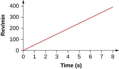
The angular velocity vs. time for a fan on a hovercraft is shown below. (a) What is the angle through which the fan blades rotate in the first 8 seconds? (b) Verify your result using the kinematic equations.
A rod of length 20 cm has two beads attached to its ends. The rod with beads starts rotating from rest. If the beads are to have a tangential speed of 20 m/s in 7 s, what is the angular acceleration of the rod to achieve this?
Show Solution
[latex]\alpha =28.6\,\text{rad}\text{/}{\text{s}}^{2}[/latex].
Glossary
- kinematics of rotational motion
- describes the relationships among rotation angle, angular velocity, angular acceleration, and time