
12 Static Equilibrium and Elasticity
12.1 Conditions for Static Equilibrium
Learning Objectives
By the end of this section, you will be able to:
- Identify the physical conditions of static equilibrium.
- Draw a free-body diagram for a rigid body acted on by forces.
- Explain how the conditions for equilibrium allow us to solve statics problems.
We say that a rigid body is in equilibrium when both its linear and angular acceleration are zero relative to an inertial frame of reference. This means that a body in equilibrium can be moving, but if so, its linear and angular velocities must be constant. We say that a rigid body is in static equilibrium when it is at rest in our selected frame of reference. Notice that the distinction between the state of rest and a state of uniform motion is artificial—that is, an object may be at rest in our selected frame of reference, yet to an observer moving at constant velocity relative to our frame, the same object appears to be in uniform motion with constant velocity. Because the motion is relative, what is in static equilibrium to us is in dynamic equilibrium to the moving observer, and vice versa. Since the laws of physics are identical for all inertial reference frames, in an inertial frame of reference, there is no distinction between static equilibrium and equilibrium.
According to Newton’s second law of motion, the linear acceleration of a rigid body is caused by a net force acting on it, or
Here, the sum is of all external forces acting on the body, where m is its mass and [latex]{\mathbf{\overset{\to }{a}}}_{\text{CM}}[/latex] is the linear acceleration of its center of mass (a concept we discussed in Linear Momentum and Collisions on linear momentum and collisions). In equilibrium, the linear acceleration is zero. If we set the acceleration to zero in Figure, we obtain the following equation:
First Equilibrium Condition
The first equilibrium condition for the static equilibrium of a rigid body expresses translational equilibrium:
The first equilibrium condition, Figure, is the equilibrium condition for forces, which we encountered when studying applications of Newton’s laws.
This vector equation is equivalent to the following three scalar equations for the components of the net force:
Analogously to Figure, we can state that the rotational acceleration [latex]\mathbf{\overset{\to }{\alpha }}[/latex] of a rigid body about a fixed axis of rotation is caused by the net torque acting on the body, or
Here [latex]I[/latex] is the rotational inertia of the body in rotation about this axis and the summation is over all torques [latex]{\mathbf{\overset{\to }{\tau }}}_{k}[/latex] of external forces in Figure. In equilibrium, the rotational acceleration is zero. By setting to zero the right-hand side of Figure, we obtain the second equilibrium condition:
Second Equilibrium Condition
The second equilibrium condition for the static equilibrium of a rigid body expresses rotational equilibrium:
The second equilibrium condition, Figure, is the equilibrium condition for torques that we encountered when we studied rotational dynamics. It is worth noting that this equation for equilibrium is generally valid for rotational equilibrium about any axis of rotation (fixed or otherwise). Again, this vector equation is equivalent to three scalar equations for the vector components of the net torque:
The second equilibrium condition means that in equilibrium, there is no net external torque to cause rotation about any axis.
The first and second equilibrium conditions are stated in a particular reference frame. The first condition involves only forces and is therefore independent of the origin of the reference frame. However, the second condition involves torque, which is defined as a cross product, [latex]{\mathbf{\overset{\to }{\tau }}}_{k}={\mathbf{\overset{\to }{r}}}_{k}\times {\mathbf{\overset{\to }{F}}}_{k},[/latex] where the position vector [latex]{\mathbf{\overset{\to }{r}}}_{k}[/latex] with respect to the axis of rotation of the point where the force is applied enters the equation. Therefore, torque depends on the location of the axis in the reference frame. However, when rotational and translational equilibrium conditions hold simultaneously in one frame of reference, then they also hold in any other inertial frame of reference, so that the net torque about any axis of rotation is still zero. The explanation for this is fairly straightforward.
Suppose vector [latex]\mathbf{\overset{\to }{R}}[/latex] is the position of the origin of a new inertial frame of reference [latex]S\prime[/latex] in the old inertial frame of reference S. From our study of relative motion, we know that in the new frame of reference [latex]S\prime ,[/latex] the position vector [latex]{{\mathbf{\overset{\to }{r}}}^{\prime }}_{k}[/latex] of the point where the force [latex]{\mathbf{\overset{\to }{F}}}_{k}[/latex] is applied is related to [latex]{\mathbf{\overset{\to }{r}}}_{k}[/latex] via the equation
Now, we can sum all torques [latex]{{\mathbf{\overset{\to }{\tau }}}^{\prime }}_{k}={{\mathbf{\overset{\to }{r}}}^{\prime }}_{k}\times {\mathbf{\overset{\to }{F}}}_{k}[/latex] of all external forces in a new reference frame, [latex]S\prime :[/latex]
In the final step in this chain of reasoning, we used the fact that in equilibrium in the old frame of reference, S, the first term vanishes because of Figure and the second term vanishes because of Figure. Hence, we see that the net torque in any inertial frame of reference [latex]S\prime[/latex] is zero, provided that both conditions for equilibrium hold in an inertial frame of reference S.
The practical implication of this is that when applying equilibrium conditions for a rigid body, we are free to choose any point as the origin of the reference frame. Our choice of reference frame is dictated by the physical specifics of the problem we are solving. In one frame of reference, the mathematical form of the equilibrium conditions may be quite complicated, whereas in another frame, the same conditions may have a simpler mathematical form that is easy to solve. The origin of a selected frame of reference is called the pivot point.
In the most general case, equilibrium conditions are expressed by the six scalar equations (Figure and Figure). For planar equilibrium problems with rotation about a fixed axis, which we consider in this chapter, we can reduce the number of equations to three. The standard procedure is to adopt a frame of reference where the z-axis is the axis of rotation. With this choice of axis, the net torque has only a z-component, all forces that have non-zero torques lie in the xy-plane, and therefore contributions to the net torque come from only the x– and y-components of external forces. Thus, for planar problems with the axis of rotation perpendicular to the xy-plane, we have the following three equilibrium conditions for forces and torques:
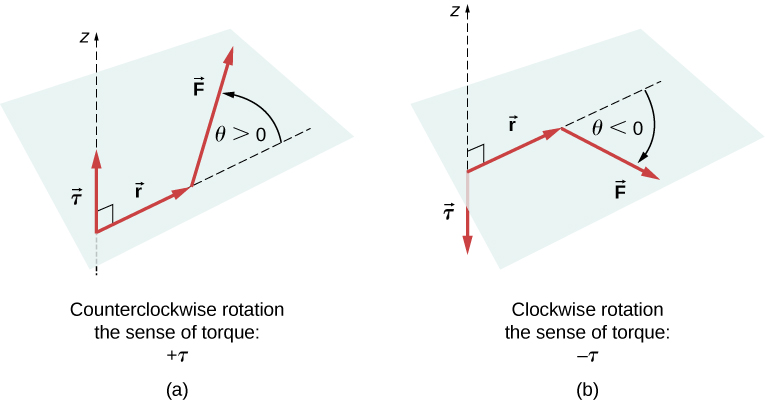
where the summation is over all N external forces acting on the body and over their torques. In Figure, we simplified the notation by dropping the subscript z, but we understand here that the summation is over all contributions along the z-axis, which is the axis of rotation. In Figure, the z-component of torque [latex]{\mathbf{\overset{\to }{\tau }}}_{k}[/latex] from the force [latex]{\mathbf{\overset{\to }{F}}}_{k}[/latex] is
where [latex]{r}_{k}[/latex] is the length of the lever arm of the force and [latex]{F}_{k}[/latex] is the magnitude of the force (as you saw in Fixed-Axis Rotation). The angle [latex]\theta[/latex] is the angle between vectors [latex]{\mathbf{\overset{\to }{r}}}_{k}[/latex] and [latex]{\mathbf{\overset{\to }{F}}}_{k},[/latex] measuring from vector [latex]{\mathbf{\overset{\to }{r}}}_{k}[/latex] to vector [latex]{\mathbf{\overset{\to }{F}}}_{k}[/latex] in the counterclockwise direction (Figure). When using Figure, we often compute the magnitude of torque and assign its sense as either positive [latex](+)[/latex] or negative [latex](-),[/latex] depending on the direction of rotation caused by this torque alone. In Figure, net torque is the sum of terms, with each term computed from Figure, and each term must have the correct sense. Similarly, in Figure, we assign the [latex]+[/latex] sign to force components in the [latex]+[/latex] x-direction and the [latex]-[/latex] sign to components in the [latex]-[/latex] x-direction. The same rule must be consistently followed in Figure, when computing force components along the y-axis.
View this demonstration to see two forces act on a rigid square in two dimensions. At all times, the static equilibrium conditions given by Figure through Figure are satisfied. You can vary magnitudes of the forces and their lever arms and observe the effect these changes have on the square.
In many equilibrium situations, one of the forces acting on the body is its weight. In free-body diagrams, the weight vector is attached to the center of gravity of the body. For all practical purposes, the center of gravity is identical to the center of mass, as you learned in Linear Momentum and Collisions on linear momentum and collisions. Only in situations where a body has a large spatial extension so that the gravitational field is nonuniform throughout its volume, are the center of gravity and the center of mass located at different points. In practical situations, however, even objects as large as buildings or cruise ships are located in a uniform gravitational field on Earth’s surface, where the acceleration due to gravity has a constant magnitude of [latex]g=9.8\,{\text{m/s}}^{2}.[/latex] In these situations, the center of gravity is identical to the center of mass. Therefore, throughout this chapter, we use the center of mass (CM) as the point where the weight vector is attached. Recall that the CM has a special physical meaning: When an external force is applied to a body at exactly its CM, the body as a whole undergoes translational motion and such a force does not cause rotation.
When the CM is located off the axis of rotation, a net gravitational torque occurs on an object. Gravitational torque is the torque caused by weight. This gravitational torque may rotate the object if there is no support present to balance it. The magnitude of the gravitational torque depends on how far away from the pivot the CM is located. For example, in the case of a tipping truck (Figure), the pivot is located on the line where the tires make contact with the road’s surface. If the CM is located high above the road’s surface, the gravitational torque may be large enough to turn the truck over. Passenger cars with a low-lying CM, close to the pavement, are more resistant to tipping over than are trucks.
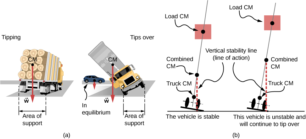
If you tilt a box so that one edge remains in contact with the table beneath it, then one edge of the base of support becomes a pivot. As long as the center of gravity of the box remains over the base of support, gravitational torque rotates the box back toward its original position of stable equilibrium. When the center of gravity moves outside of the base of support, gravitational torque rotates the box in the opposite direction, and the box rolls over. View this demonstration to experiment with stable and unstable positions of a box.
Example
Center of Gravity of a Car
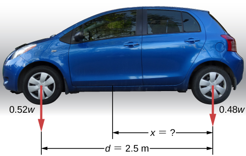
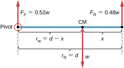
A passenger car with a 2.5-m wheelbase has 52% of its weight on the front wheels on level ground, as illustrated in Figure. Where is the CM of this car located with respect to the rear axle?
Strategy
We do not know the weight w of the car. All we know is that when the car rests on a level surface, 0.52w pushes down on the surface at contact points of the front wheels and 0.48w pushes down on the surface at contact points of the rear wheels. Also, the contact points are separated from each other by the distance [latex]d=2.5\,\text{m}.[/latex] At these contact points, the car experiences normal reaction forces with magnitudes [latex]{F}_{\text{F}}=0.52w[/latex] and [latex]{F}_{\text{R}}=0.48w[/latex] on the front and rear axles, respectively. We also know that the car is an example of a rigid body in equilibrium whose entire weight w acts at its CM. The CM is located somewhere between the points where the normal reaction forces act, somewhere at a distance x from the point where [latex]{F}_{R}[/latex] acts. Our task is to find x. Thus, we identify three forces acting on the body (the car), and we can draw a free-body diagram for the extended rigid body, as shown in Figure.
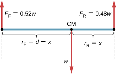
We are almost ready to write down equilibrium conditions Figure through Figure for the car, but first we must decide on the reference frame. Suppose we choose the x-axis along the length of the car, the y-axis vertical, and the z-axis perpendicular to this xy-plane. With this choice we only need to write Figure and Figure because all the y-components are identically zero. Now we need to decide on the location of the pivot point. We can choose any point as the location of the axis of rotation (z-axis). Suppose we place the axis of rotation at CM, as indicated in the free-body diagram for the car. At this point, we are ready to write the equilibrium conditions for the car.
Solution
Each equilibrium condition contains only three terms because there are [latex]N=3[/latex] forces acting on the car. The first equilibrium condition, Figure, reads
This condition is trivially satisfied because when we substitute the data, Figure becomes [latex]+0.52w-w+0.48w=0.[/latex] The second equilibrium condition, Figure, reads
where [latex]{\tau }_{\text{F}}[/latex] is the torque of force [latex]{F}_{\text{F}},\,{\tau }_{w}[/latex] is the gravitational torque of force w, and [latex]{\tau }_{\text{R}}[/latex] is the torque of force [latex]{F}_{\text{R}}.[/latex] When the pivot is located at CM, the gravitational torque is identically zero because the lever arm of the weight with respect to an axis that passes through CM is zero. The lines of action of both normal reaction forces are perpendicular to their lever arms, so in Figure, we have [latex]|\,\text{sin}\,\theta |=1[/latex] for both forces. From the free-body diagram, we read that torque [latex]{\tau }_{\text{F}}[/latex] causes clockwise rotation about the pivot at CM, so its sense is negative; and torque [latex]{\tau }_{\text{R}}[/latex] causes counterclockwise rotation about the pivot at CM, so its sense is positive. With this information, we write the second equilibrium condition as
With the help of the free-body diagram, we identify the force magnitudes [latex]{F}_{\text{R}}=0.48w[/latex] and [latex]{F}_{\text{F}}=0.52w,[/latex] and their corresponding lever arms [latex]{r}_{\text{R}}=x[/latex] and [latex]{r}_{\text{F}}=d-x.[/latex] We can now write the second equilibrium condition, Figure, explicitly in terms of the unknown distance x:
Here the weight w cancels and we can solve the equation for the unknown position x of the CM. The answer is [latex]x=0.52d=0.52(2.5\,\text{m})=1.3\,\text{m}\text{.}[/latex]
Solution
Choosing the pivot at the position of the front axle does not change the result. The free-body diagram for this pivot location is presented in Figure. For this choice of pivot point, the second equilibrium condition is
When we substitute the quantities indicated in the diagram, we obtain
The answer obtained by solving Figure is, again, [latex]x=0.52d=1.3\,\text{m}.[/latex]
Significance
This example shows that when solving static equilibrium problems, we are free to choose the pivot location. For different choices of the pivot point we have different sets of equilibrium conditions to solve. However, all choices lead to the same solution to the problem.
Check Your Understanding
Solve Figure by choosing the pivot at the location of the rear axle.
Show Solution
[latex]x=1.3\,\text{m}[/latex]
Check Your Understanding
Explain which one of the following situations satisfies both equilibrium conditions: (a) a tennis ball that does not spin as it travels in the air; (b) a pelican that is gliding in the air at a constant velocity at one altitude; or (c) a crankshaft in the engine of a parked car.
Show Solution
(b), (c)
A special case of static equilibrium occurs when all external forces on an object act at or along the axis of rotation or when the spatial extension of the object can be disregarded. In such a case, the object can be effectively treated like a point mass. In this special case, we need not worry about the second equilibrium condition, Figure, because all torques are identically zero and the first equilibrium condition (for forces) is the only condition to be satisfied. The free-body diagram and problem-solving strategy for this special case were outlined in Newton’s Laws of Motion and Applications of Newton’s Laws. You will see a typical equilibrium situation involving only the first equilibrium condition in the next example.
View this demonstration to see three weights that are connected by strings over pulleys and tied together in a knot. You can experiment with the weights to see how they affect the equilibrium position of the knot and, at the same time, see the vector-diagram representation of the first equilibrium condition at work.
Example
A Breaking Tension
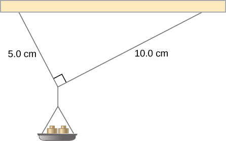
A small pan of mass 42.0 g is supported by two strings, as shown in Figure. The maximum tension that the string can support is 2.80 N. Mass is added gradually to the pan until one of the strings snaps. Which string is it? How much mass must be added for this to occur?
Strategy
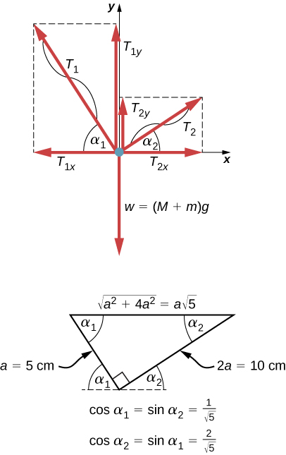
This mechanical system consisting of strings, masses, and the pan is in static equilibrium. Specifically, the knot that ties the strings to the pan is in static equilibrium. The knot can be treated as a point; therefore, we need only the first equilibrium condition. The three forces pulling at the knot are the tension [latex]{\mathbf{\overset{\to }{T}}}_{1}[/latex] in the 5.0-cm string, the tension [latex]{\mathbf{\overset{\to }{T}}}_{2}[/latex] in the 10.0-cm string, and the weight [latex]\mathbf{\overset{\to }{w}}[/latex] of the pan holding the masses. We adopt a rectangular coordinate system with the y-axis pointing opposite to the direction of gravity and draw the free-body diagram for the knot (see Figure). To find the tension components, we must identify the direction angles [latex]{\alpha }_{1}[/latex] and [latex]{\alpha }_{2}[/latex] that the strings make with the horizontal direction that is the x-axis. As you can see in Figure, the strings make two sides of a right triangle. We can use the Pythagorean theorem to solve this triangle, shown in Figure, and find the sine and cosine of the angles [latex]{\alpha }_{1}[/latex] and [latex]{\alpha }_{2}.[/latex] Then we can resolve the tensions into their rectangular components, substitute in the first condition for equilibrium (Figure and Figure), and solve for the tensions in the strings. The string with a greater tension will break first.
Solution
The weight w pulling on the knot is due to the mass M of the pan and mass m added to the pan, or [latex]w=(M+m)g.[/latex] With the help of the free-body diagram in Figure, we can set up the equilibrium conditions for the knot:
From the free-body diagram, the magnitudes of components in these equations are
We substitute these components into the equilibrium conditions and simplify. We then obtain two equilibrium equations for the tensions:
The equilibrium equation for the x-direction tells us that the tension [latex]{T}_{1}[/latex] in the 5.0-cm string is twice the tension [latex]{T}_{2}[/latex] in the 10.0-cm string. Therefore, the shorter string will snap. When we use the first equation to eliminate [latex]{T}_{2}[/latex] from the second equation, we obtain the relation between the mass [latex]m[/latex] on the pan and the tension [latex]{T}_{1}[/latex] in the shorter string:
The string breaks when the tension reaches the critical value of [latex]{T}_{1}=2.80\,\text{N}.[/latex] The preceding equation can be solved for the critical mass m that breaks the string:
Significance
Suppose that the mechanical system considered in this example is attached to a ceiling inside an elevator going up. As long as the elevator moves up at a constant speed, the result stays the same because the weight [latex]w[/latex] does not change. If the elevator moves up with acceleration, the critical mass is smaller because the weight of [latex]M+m[/latex] becomes larger by an apparent weight due to the acceleration of the elevator. Still, in all cases the shorter string breaks first.
Summary
- A body is in equilibrium when it remains either in uniform motion (both translational and rotational) or at rest. When a body in a selected inertial frame of reference neither rotates nor moves in translational motion, we say the body is in static equilibrium in this frame of reference.
- Conditions for equilibrium require that the sum of all external forces acting on the body is zero (first condition of equilibrium), and the sum of all external torques from external forces is zero (second condition of equilibrium). These two conditions must be simultaneously satisfied in equilibrium. If one of them is not satisfied, the body is not in equilibrium.
- The free-body diagram for a body is a useful tool that allows us to count correctly all contributions from all external forces and torques acting on the body. Free-body diagrams for the equilibrium of an extended rigid body must indicate a pivot point and lever arms of acting forces with respect to the pivot.
Conceptual Questions
What can you say about the velocity of a moving body that is in dynamic equilibrium?
Show Solution
constant
Under what conditions can a rotating body be in equilibrium? Give an example.
What three factors affect the torque created by a force relative to a specific pivot point?
Show Solution
magnitude and direction of the force, and its lever arm
Mechanics sometimes put a length of pipe over the handle of a wrench when trying to remove a very tight bolt. How does this help?
For the next four problems, evaluate the statement as either true or false and explain your answer.
If there is only one external force (or torque) acting on an object, it cannot be in equilibrium.
Show Solution
True, as the sum of forces cannot be zero in this case unless the force itself is zero.
If an object is in equilibrium there must be an even number of forces acting on it.
If an odd number of forces act on an object, the object cannot be in equilibrium.
Show Solution
False, provided forces add to zero as vectors then equilibrium can be achieved.
A body moving in a circle with a constant speed is in rotational equilibrium.
What purpose is served by a long and flexible pole carried by wire-walkers?
Show Solution
It helps a wire-walker to maintain equilibrium.
Problems
When tightening a bolt, you push perpendicularly on a wrench with a force of 165 N at a distance of 0.140 m from the center of the bolt. How much torque are you exerting relative to the center of the bolt?
When opening a door, you push on it perpendicularly with a force of 55.0 N at a distance of 0.850 m from the hinges. What torque are you exerting relative to the hinges?
Show Solution
[latex]46.8\,\text{N}\cdot \text{m}[/latex]
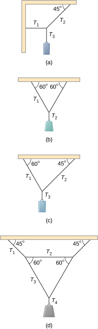
Find the magnitude of the tension in each supporting cable shown below. In each case, the weight of the suspended body is 100.0 N and the masses of the cables are negligible.
What force must be applied at point P to keep the structure shown in equilibrium? The weight of the structure is negligible.
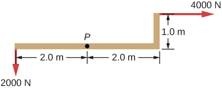
153.4°Show Answer
Is it possible to apply a force at P to keep in equilibrium the structure shown? The weight of the structure is negligible.

Two children push on opposite sides of a door during play. Both push horizontally and perpendicular to the door. One child pushes with a force of 17.5 N at a distance of 0.600 m from the hinges, and the second child pushes at a distance of 0.450 m. What force must the second child exert to keep the door from moving? Assume friction is negligible.
Show Solution
23.3 N
A small 1000-kg SUV has a wheel base of 3.0 m. If 60% if its weight rests on the front wheels, how far behind the front wheels is the wagon’s center of mass?
The uniform seesaw is balanced at its center of mass, as seen below. The smaller boy on the right has a mass of 40.0 kg. What is the mass of his friend?
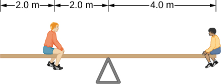
80.0 kgShow Answer
Glossary
- center of gravity
- point where the weight vector is attached
- equilibrium
- body is in equilibrium when its linear and angular accelerations are both zero relative to an inertial frame of reference
- first equilibrium condition
- expresses translational equilibrium; all external forces acting on the body balance out and their vector sum is zero
- gravitational torque
- torque on the body caused by its weight; it occurs when the center of gravity of the body is not located on the axis of rotation
- second equilibrium condition
- expresses rotational equilibrium; all torques due to external forces acting on the body balance out and their vector sum is zero
- static equilibrium
- body is in static equilibrium when it is at rest in our selected inertial frame of reference