
4 Motion in Two and Three Dimensions
4.1 Displacement and Velocity Vectors
Learning Objectives
By the end of this section, you will be able to:
- Calculate position vectors in a multidimensional displacement problem.
- Solve for the displacement in two or three dimensions.
- Calculate the velocity vector given the position vector as a function of time.
- Calculate the average velocity in multiple dimensions.
Displacement and velocity in two or three dimensions are straightforward extensions of the one-dimensional definitions. However, now they are vector quantities, so calculations with them have to follow the rules of vector algebra, not scalar algebra.
Displacement Vector
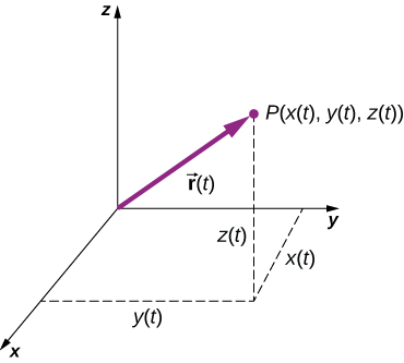
To describe motion in two and three dimensions, we must first establish a coordinate system and a convention for the axes. We generally use the coordinates x, y, and z to locate a particle at point P(x, y, z) in three dimensions. If the particle is moving, the variables x, y, and z are functions of time (t):
The position vector from the origin of the coordinate system to point P is [latex]\mathbf{\overset{\to }{r}}(t).[/latex] In unit vector notation, introduced in Coordinate Systems and Components of a Vector, [latex]\mathbf{\overset{\to }{r}}(t)[/latex] is
Figure shows the coordinate system and the vector to point P, where a particle could be located at a particular time t. Note the orientation of the x, y, and z axes. This orientation is called a right-handed coordinate system (Coordinate Systems and Components of a Vector) and it is used throughout the chapter.
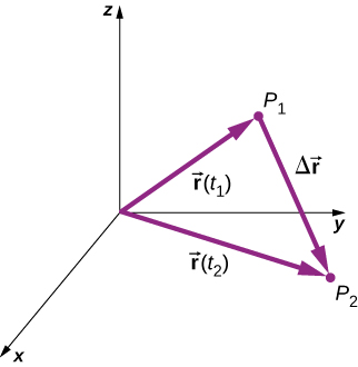
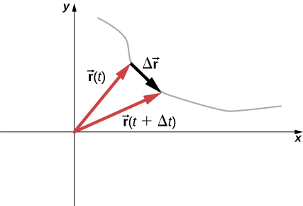
With our definition of the position of a particle in three-dimensional space, we can formulate the three-dimensional displacement. Figure shows a particle at time [latex]{t}_{1}[/latex] located at [latex]{P}_{1}[/latex] with position vector [latex]\mathbf{\overset{\to }{r}}({t}_{1}).[/latex] At a later time [latex]{t}_{2},[/latex] the particle is located at [latex]{P}_{2}[/latex] with position vector [latex]\mathbf{\overset{\to }{r}}({t}_{2})[/latex]. The displacement vector [latex]\Delta \mathbf{\overset{\to }{r}}[/latex] is found by subtracting [latex]\mathbf{\overset{\to }{r}}({t}_{1})[/latex] from [latex]\mathbf{\overset{\to }{r}}({t}_{2})\text{ }:[/latex]
Vector addition is discussed in Vectors. Note that this is the same operation we did in one dimension, but now the vectors are in three-dimensional space.
The following examples illustrate the concept of displacement in multiple dimensions.
Example
Polar Orbiting Satellite
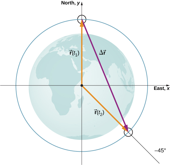
A satellite is in a circular polar orbit around Earth at an altitude of 400 km—meaning, it passes directly overhead at the North and South Poles. What is the magnitude and direction of the displacement vector from when it is directly over the North Pole to when it is at [latex]-45^\circ[/latex] latitude?
Strategy
We make a picture of the problem to visualize the solution graphically. This will aid in our understanding of the displacement. We then use unit vectors to solve for the displacement.
Solution
Show Answer
Figure shows the surface of Earth and a circle that represents the orbit of the satellite. Although satellites are moving in three-dimensional space, they follow trajectories of ellipses, which can be graphed in two dimensions. The position vectors are drawn from the center of Earth, which we take to be the origin of the coordinate system, with the y-axis as north and the x-axis as east. The vector between them is the displacement of the satellite. We take the radius of Earth as 6370 km, so the length of each position vector is 6770 km.
In unit vector notation, the position vectors are
Evaluating the sine and cosine, we have
Now we can find [latex]\Delta \mathbf{\overset{\to }{r}}[/latex], the displacement of the satellite:
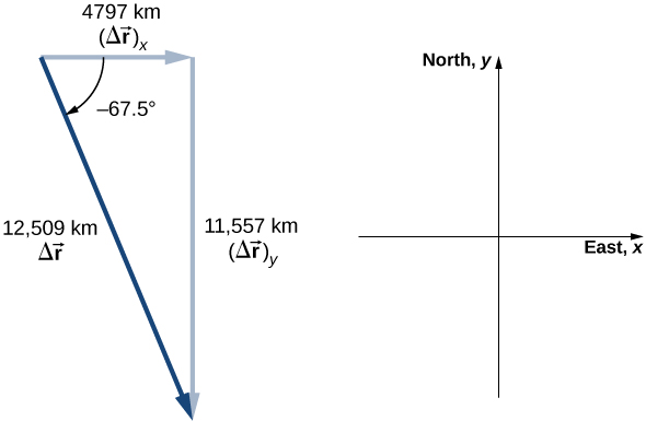
The magnitude of the displacement is [latex]|\Delta \mathbf{\overset{\to }{r}}|=\sqrt{{(4787)}^{2}+{(-11,557)}^{2}}=12,509\,\text{km}.[/latex] The angle the displacement makes with the x-axis is [latex]\theta ={\text{tan}}^{-1}(\frac{-11,557}{4787})=-67.5^\circ.[/latex]
Significance
Plotting the displacement gives information and meaning to the unit vector solution to the problem. When plotting the displacement, we need to include its components as well as its magnitude and the angle it makes with a chosen axis—in this case, the x-axis (Figure).
Note that the satellite took a curved path along its circular orbit to get from its initial position to its final position in this example. It also could have traveled 4787 km east, then 11,557 km south to arrive at the same location. Both of these paths are longer than the length of the displacement vector. In fact, the displacement vector gives the shortest path between two points in one, two, or three dimensions.
Many applications in physics can have a series of displacements, as discussed in the previous chapter. The total displacement is the sum of the individual displacements, only this time, we need to be careful, because we are adding vectors. We illustrate this concept with an example of Brownian motion.
Example
Brownian Motion
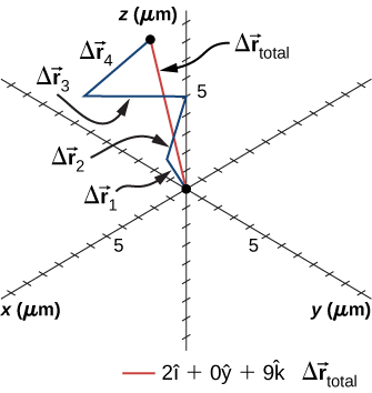
Brownian motion is a chaotic random motion of particles suspended in a fluid, resulting from collisions with the molecules of the fluid. This motion is three-dimensional. The displacements in numerical order of a particle undergoing Brownian motion could look like the following, in micrometers (Figure):
What is the total displacement of the particle from the origin?
Solution
Show Answer
We form the sum of the displacements and add them as vectors:
[latex]\begin{array}{cc}\hfill \Delta {\mathbf{\overset{\to }{r}}}_{\text{Total}}& =\sum \Delta {\mathbf{\overset{\to }{r}}}_{i}=\Delta {\mathbf{\overset{\to }{r}}}_{1}+\Delta {\mathbf{\overset{\to }{r}}}_{2}+\Delta {\mathbf{\overset{\to }{r}}}_{3}+\Delta {\mathbf{\overset{\to }{r}}}_{4}\hfill \\ & =(2.0-1.0+4.0-3.0)\mathbf{\hat{i}}+(1.0+0-2.0+1.0)\mathbf{\hat{j}}+(3.0+3.0+1.0+2.0)\mathbf{\hat{k}}\hfill \\ & =2.0\mathbf{\hat{i}}+0\mathbf{\hat{j}}+9.0\mathbf{\hat{k}}\mu \text{m}.\hfill \end{array}[/latex]
To complete the solution, we express the displacement as a magnitude and direction,
[latex]|\Delta {\mathbf{\overset{\to }{r}}}_{\text{Total}}|=\sqrt{{2.0}^{2}+{0}^{2}+{9.0}^{2}}=9.2\,\mu \text{m,}\quad \theta ={\text{tan}}^{-1}(\frac{9}{2})=77^\circ,[/latex]
with respect to the x-axis in the xz-plane.
Significance
From the figure we can see the magnitude of the total displacement is less than the sum of the magnitudes of the individual displacements.
Velocity Vector
In the previous chapter we found the instantaneous velocity by calculating the derivative of the position function with respect to time. We can do the same operation in two and three dimensions, but we use vectors. The instantaneous velocity vector is now
Let’s look at the relative orientation of the position vector and velocity vector graphically. In Figure we show the vectors [latex]\mathbf{\overset{\to }{r}}(t)[/latex] and [latex]\mathbf{\overset{\to }{r}}(t+\Delta t),[/latex] which give the position of a particle moving along a path represented by the gray line. As [latex]\Delta t[/latex] goes to zero, the velocity vector, given by Figure, becomes tangent to the path of the particle at time t.
(Equation) can also be written in terms of the components of [latex]\mathbf{\overset{\to }{v}}(t).[/latex] Since
we can write
where
If only the average velocity is of concern, we have the vector equivalent of the one-dimensional average velocity for two and three dimensions:
Example
Calculating the Velocity Vector
The position function of a particle is [latex]\mathbf{\overset{\to }{r}}(t)=2.0{t}^{2}\mathbf{\hat{i}}+(2.0+3.0t)\mathbf{\hat{j}}+5.0t\mathbf{\hat{k}}\text{m}.[/latex] (a) What is the instantaneous velocity and speed at t = 2.0 s? (b) What is the average velocity between 1.0 s and 3.0 s?
Solution
Using Figure and Figure, and taking the derivative of the position function with respect to time, we find
Show Answer
(a) [latex]v(t)=\frac{d\mathbf{\text{r}}(t)}{dt}=4.0t\mathbf{\hat{i}}+3.0\mathbf{\hat{j}}+5.0\mathbf{\hat{k}}\text{m/s}[/latex] [latex]\mathbf{\overset{\to }{v}}(2.0s)=8.0\mathbf{\hat{i}}+3.0\mathbf{\hat{j}}+5.0\mathbf{\hat{k}}\text{m/s}[/latex] Speed [latex]|\mathbf{\overset{\to }{v}}(2.0\,\text{s})|=\sqrt{{8}^{2}+{3}^{2}+{5}^{2}}=9.9\,\text{m/s}.[/latex]
(b)
Show Answer
From Figure,
[latex]\begin{array}{cc}\hfill {\mathbf{\overset{\to }{v}}}_{\text{avg}}& =\frac{\mathbf{\overset{\to }{r}}({t}_{2})-\mathbf{\overset{\to }{r}}({t}_{1})}{{t}_{2}-{t}_{1}}=\frac{\mathbf{\overset{\to }{r}}(3.0\,\text{s})-\mathbf{\overset{\to }{r}}(1.0\,\text{s})}{3.0\,\text{s}-1.0\,\text{s}}=\frac{(18\mathbf{\hat{i}}+11\mathbf{\hat{j}}+15\mathbf{\hat{k}})\,\text{m}-(2\mathbf{\hat{i}}+5\mathbf{\hat{j}}+5\mathbf{\hat{k}})\,\text{m}}{2.0\,\text{s}}\hfill \\ & =\frac{(16\mathbf{\hat{i}}+6\mathbf{\hat{j}}+10\mathbf{\hat{k}})\,\text{m}}{2.0\,\text{s}}=8.0\mathbf{\hat{i}}+3.0\mathbf{\hat{j}}+5.0\mathbf{\hat{k}}\text{m/s}.\hfill \end{array}[/latex]
Significance
We see the average velocity is the same as the instantaneous velocity at t = 2.0 s, as a result of the velocity function being linear. This need not be the case in general. In fact, most of the time, instantaneous and average velocities are not the same.
Check Your Understanding
The position function of a particle is [latex]\mathbf{\overset{\to }{r}}(t)=3.0{t}^{3}\mathbf{\hat{i}}+4.0\mathbf{\hat{j}}.[/latex] (a) What is the instantaneous velocity at t = 3 s? (b) Is the average velocity between 2 s and 4 s equal to the instantaneous velocity at t = 3 s?
Show Solution
(a) Taking the derivative with respect to time of the position function, we have [latex]\mathbf{\overset{\to }{v}}(t)=9.0{t}^{2}\mathbf{\hat{i}}\text{and}\mathbf{\overset{\to }{v}}\text{(3.0s)}=81.0\mathbf{\hat{i}}\text{m/s}.[/latex] (b) Since the velocity function is nonlinear, we suspect the average velocity is not equal to the instantaneous velocity. We check this and find
[latex]{\mathbf{\overset{\to }{v}}}_{\text{avg}}=\frac{\mathbf{\overset{\to }{r}}({t}_{2})-\mathbf{\overset{\to }{r}}({t}_{1})}{{t}_{2}-{t}_{1}}=\frac{\mathbf{\overset{\to }{r}}(4.0\,\text{s})-\mathbf{\overset{\to }{r}}(2.0\,\text{s})}{4.0\,\text{s}-2.0\,\text{s}}=\frac{(144.0\mathbf{\hat{i}}-36.0\mathbf{\hat{i}})\,\text{m}}{2.0\,\text{s}}=54.0\mathbf{\hat{i}}\text{m/s},[/latex]
which is different from [latex]\mathbf{\overset{\to }{v}}\text{(3.0s)}=81.0\mathbf{\hat{i}}\text{m/s}.[/latex]
The Independence of Perpendicular Motions
When we look at the three-dimensional equations for position and velocity written in unit vector notation, Figure and Figure, we see the components of these equations are separate and unique functions of time that do not depend on one another. Motion along the x direction has no part of its motion along the y and z directions, and similarly for the other two coordinate axes. Thus, the motion of an object in two or three dimensions can be divided into separate, independent motions along the perpendicular axes of the coordinate system in which the motion takes place.
To illustrate this concept with respect to displacement, consider a woman walking from point A to point B in a city with square blocks. The woman taking the path from A to B may walk east for so many blocks and then north (two perpendicular directions) for another set of blocks to arrive at B. How far she walks east is affected only by her motion eastward. Similarly, how far she walks north is affected only by her motion northward.
In the kinematic description of motion, we are able to treat the horizontal and vertical components of motion separately. In many cases, motion in the horizontal direction does not affect motion in the vertical direction, and vice versa.
An example illustrating the independence of vertical and horizontal motions is given by two baseballs. One baseball is dropped from rest. At the same instant, another is thrown horizontally from the same height and it follows a curved path. A stroboscope captures the positions of the balls at fixed time intervals as they fall (Figure).
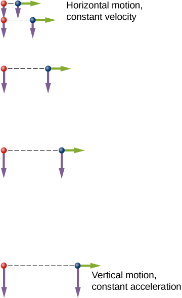
It is remarkable that for each flash of the strobe, the vertical positions of the two balls are the same. This similarity implies vertical motion is independent of whether the ball is moving horizontally. (Assuming no air resistance, the vertical motion of a falling object is influenced by gravity only, not by any horizontal forces.) Careful examination of the ball thrown horizontally shows it travels the same horizontal distance between flashes. This is because there are no additional forces on the ball in the horizontal direction after it is thrown. This result means horizontal velocity is constant and is affected neither by vertical motion nor by gravity (which is vertical). Note this case is true for ideal conditions only. In the real world, air resistance affects the speed of the balls in both directions.
The two-dimensional curved path of the horizontally thrown ball is composed of two independent one-dimensional motions (horizontal and vertical). The key to analyzing such motion, called projectile motion, is to resolve it into motions along perpendicular directions. Resolving two-dimensional motion into perpendicular components is possible because the components are independent.
Summary
- The position function [latex]\mathbf{\overset{\to }{r}}(t)[/latex] gives the position as a function of time of a particle moving in two or three dimensions. Graphically, it is a vector from the origin of a chosen coordinate system to the point where the particle is located at a specific time.
- The displacement vector [latex]\Delta \mathbf{\overset{\to }{r}}[/latex] gives the shortest distance between any two points on the trajectory of a particle in two or three dimensions.
- Instantaneous velocity gives the speed and direction of a particle at a specific time on its trajectory in two or three dimensions, and is a vector in two and three dimensions.
- The velocity vector is tangent to the trajectory of the particle.
- Displacement [latex]\mathbf{\overset{\to }{r}}(t)[/latex] can be written as a vector sum of the one-dimensional displacements [latex]\mathbf{\overset{\to }{x}}(t),\mathbf{\overset{\to }{y}}(t),\mathbf{\overset{\to }{z}}(t)[/latex] along the x, y, and z directions.
- Velocity [latex]\mathbf{\overset{\to }{v}}(t)[/latex] can be written as a vector sum of the one-dimensional velocities [latex]{v}_{x}(t),{v}_{y}(t),{v}_{z}(t)[/latex] along the x, y, and z directions.
- Motion in any given direction is independent of motion in a perpendicular direction.
Conceptual Questions
What form does the trajectory of a particle have if the distance from any point A to point B is equal to the magnitude of the displacement from A to B?
Show Solution
straight line
Give an example of a trajectory in two or three dimensions caused by independent perpendicular motions.
If the instantaneous velocity is zero, what can be said about the slope of the position function?
Show Solution
The slope must be zero because the velocity vector is tangent to the graph of the position function.
Problems
The coordinates of a particle in a rectangular coordinate system are (1.0, –4.0, 6.0). What is the position vector of the particle?
Show Solution
[latex]\mathbf{\overset{\to }{r}}=1.0\mathbf{\hat{i}}-4.0\mathbf{\hat{j}}+6.0\mathbf{\hat{k}}[/latex]
The position of a particle changes from [latex]{\mathbf{\overset{\to }{r}}}_{1}=(2.0\text{}\mathbf{\hat{i}}+3.0\mathbf{\hat{j}})\text{cm}[/latex] to [latex]{\mathbf{\overset{\to }{r}}}_{2}=(-4.0\mathbf{\hat{i}}+3.0\mathbf{\hat{j}})\,\text{cm}.[/latex] What is the particle’s displacement?
The 18th hole at Pebble Beach Golf Course is a dogleg to the left of length 496.0 m. The fairway off the tee is taken to be the x direction. A golfer hits his tee shot a distance of 300.0 m, corresponding to a displacement [latex]\Delta {\mathbf{\overset{\to }{r}}}_{1}=300.0\,\text{m}\mathbf{\hat{i}},[/latex] and hits his second shot 189.0 m with a displacement [latex]\Delta {\mathbf{\overset{\to }{r}}}_{2}=172.0\,\text{m}\mathbf{\hat{i}}+80.3\,\text{m}\mathbf{\hat{j}}.[/latex] What is the final displacement of the golf ball from the tee?
Show Solution
[latex]\Delta {\mathbf{\overset{\to }{r}}}_{\text{Total}}=472.0\,\text{m}\mathbf{\hat{i}}+80.3\,\text{m}\mathbf{\hat{j}}[/latex]
A bird flies straight northeast a distance of 95.0 km for 3.0 h. With the x-axis due east and the y-axis due north, what is the displacement in unit vector notation for the bird? What is the average velocity for the trip?
A cyclist rides 5.0 km due east, then 10.0 km [latex]20^\circ[/latex] west of north. From this point she rides 8.0 km due west. What is the final displacement from where the cyclist started?
Show Solution
[latex]\text{Sum of displacements}=-6.4\,\text{km}\mathbf{\hat{i}}+9.4\,\text{km}\mathbf{\hat{j}}[/latex]
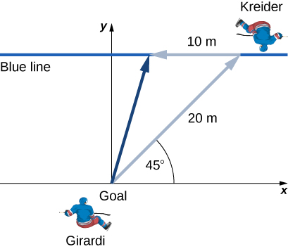
New York Rangers defenseman Daniel Girardi stands at the goal and passes a hockey puck 20 m and [latex]45^\circ[/latex] from straight down the ice to left wing Chris Kreider waiting at the blue line. Kreider waits for Girardi to reach the blue line and passes the puck directly across the ice to him 10 m away. What is the final displacement of the puck? See the following figure.
The position of a particle is [latex]\mathbf{\overset{\to }{r}}(t)=4.0{t}^{2}\mathbf{\hat{i}}-3.0\mathbf{\hat{j}}+2.0{t}^{3}\mathbf{\hat{k}}\text{m}.[/latex] (a) What is the velocity of the particle at 0 s and at [latex]1.0[/latex] s? (b) What is the average velocity between 0 s and [latex]1.0[/latex] s?
Show Solution
a. [latex]\mathbf{\overset{\to }{v}}(t)=8.0t\mathbf{\hat{i}}+6.0{t}^{2}\mathbf{\hat{k}},\enspace\mathbf{\overset{\to }{v}}(0)=0,\enspace\mathbf{\overset{\to }{v}}(1.0)=8.0\mathbf{\hat{i}}+6.0\mathbf{\hat{k}}\text{m/s}[/latex],
b. [latex]{\mathbf{\overset{\to }{v}}}_{\text{avg}}=4.0\text{}\mathbf{\hat{i}}+2.0\mathbf{\hat{k}}\,\text{m/s}[/latex]
Clay Matthews, a linebacker for the Green Bay Packers, can reach a speed of 10.0 m/s. At the start of a play, Matthews runs downfield at [latex]45^\circ[/latex] with respect to the 50-yard line and covers 8.0 m in 1 s. He then runs straight down the field at [latex]90^\circ[/latex] with respect to the 50-yard line for 12 m, with an elapsed time of 1.2 s. (a) What is Matthews’ final displacement from the start of the play? (b) What is his average velocity?
The F-35B Lighting II is a short-takeoff and vertical landing fighter jet. If it does a vertical takeoff to 20.00-m height above the ground and then follows a flight path angled at [latex]30^\circ[/latex] with respect to the ground for 20.00 km, what is the final displacement?
Show Solution
[latex]\Delta {\mathbf{\overset{\to }{r}}}_{1}=20.00\,\text{m}\mathbf{\hat{j}},\Delta {\mathbf{\overset{\to }{r}}}_{2}=(2.000\times {10}^{4}\text{m})\,(\text{cos}30^\circ\mathbf{\hat{i}}+\text{sin}\,30^\circ\mathbf{\hat{j}})[/latex]
[latex]\Delta \mathbf{\overset{\to }{r}}=1.700\times {10}^{4}\text{m}\mathbf{\hat{i}}+1.002\times {10}^{4}\text{m}\mathbf{\hat{j}}[/latex]
Glossary
- displacement vector
- vector from the initial position to a final position on a trajectory of a particle
- position vector
- vector from the origin of a chosen coordinate system to the position of a particle in two- or three-dimensional space
- velocity vector
- vector that gives the instantaneous speed and direction of a particle; tangent to the trajectory