The Quantum Tunneling of Particles through Potential Barriers

Samuel J. Ling; Jeff Sanny; William Moebs

Quantum Mechanics

The Quantum Tunneling of Particles through Potential Barriers

Samuel J. Ling; Jeff Sanny; and William Moebs

Learning Objectives

By the end of this section, you will be able to:

Describe how a quantum particle may tunnel across a potential barrier
Identify important physical parameters that affect the tunneling probability
Identify the physical phenomena where quantum tunneling is observed
Explain how quantum tunneling is utilized in modern technologies

Quantum tunneling is a phenomenon in which particles penetrate a potential energy barrier with a height greater than the total energy of the particles. The phenomenon is interesting and important because it violates the principles of classical mechanics. Quantum tunneling is important in models of the Sun and has a wide range of applications, such as the scanning tunneling microscope and the tunnel diode.

Tunneling and Potential Energy

To illustrate quantum tunneling, consider a ball rolling along a surface with a kinetic energy of 100 J. As the ball rolls, it encounters a hill. The potential energy of the ball placed atop the hill is 10 J. Therefore, the ball (with 100 J of kinetic energy) easily rolls over the hill and continues on. In classical mechanics, the probability that the ball passes over the hill is exactly 1—it makes it over every time. If, however, the height of the hill is increased—a ball placed atop the hill has a potential energy of 200 J—the ball proceeds only part of the way up the hill, stops, and returns in the direction it came. The total energy of the ball is converted entirely into potential energy before it can reach the top of the hill. We do not expect, even after repeated attempts, for the 100-J ball to ever be found beyond the hill. Therefore, the probability that the ball passes over the hill is exactly 0, and probability it is turned back or “reflected” by the hill is exactly 1. The ball never makes it over the hill. The existence of the ball beyond the hill is an impossibility or “energetically forbidden.”

However, according to quantum mechanics, the ball has a wave function and this function is defined over all space. The wave function may be highly localized, but there is always a chance that as the ball encounters the hill, the ball will suddenly be found beyond it. Indeed, this probability is appreciable if the “wave packet” of the ball is wider than the barrier.

View this interactive simulation for a simulation of tunneling.

In the language of quantum mechanics, the hill is characterized by a potential barrier. A finite-height square barrier is described by the following potential-energy function:

$U\left(x\right)=\left\{\begin{array}{cc}\hfill 0,& \text{when}\phantom{\rule{0.2em}{0ex}}x<0\hfill \\ \hfill {U}_{0},& \text{when}\phantom{\rule{0.2em}{0ex}}0\le x\le L\hfill \\ \hfill 0,& \text{when}\phantom{\rule{0.2em}{0ex}}x>L.\hfill \end{array}$

The potential barrier is illustrated in (Figure). When the height ${U}_{0}$ of the barrier is infinite, the wave packet representing an incident quantum particle is unable to penetrate it, and the quantum particle bounces back from the barrier boundary, just like a classical particle. When the width L of the barrier is infinite and its height is finite, a part of the wave packet representing an incident quantum particle can filter through the barrier boundary and eventually perish after traveling some distance inside the barrier.

A potential energy barrier of height ${U}_{0}$ creates three physical regions with three different wave behaviors. In region I where $x<0$ , an incident wave packet (incident particle) moves in a potential-free zone and coexists with a reflected wave packet (reflected particle). In region II, a part of the incident wave that has not been reflected at $x=0$ moves as a transmitted wave in a constant potential $U\left(x\right)=+{U}_{0}$ and tunnels through to region III at $x=L$ . In region III for $x>L$ , a wave packet (transmitted particle) that has tunneled through the potential barrier moves as a free particle in potential-free zone. The energy E of the incident particle is indicated by the horizontal line.

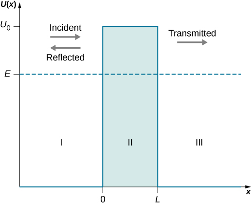
When both the width L and the height ${U}_{0}$ are finite, a part of the quantum wave packet incident on one side of the barrier can penetrate the barrier boundary and continue its motion inside the barrier, where it is gradually attenuated on its way to the other side. A part of the incident quantum wave packet eventually emerges on the other side of the barrier in the form of the transmitted wave packet that tunneled through the barrier. How much of the incident wave can tunnel through a barrier depends on the barrier width L and its height ${U}_{0}$ , and on the energy E of the quantum particle incident on the barrier. This is the physics of tunneling.

Barrier penetration by quantum wave functions was first analyzed theoretically by Friedrich Hund in 1927, shortly after Schrӧdinger published the equation that bears his name. A year later, George Gamow used the formalism of quantum mechanics to explain the radioactive $\text{α}$ -decay of atomic nuclei as a quantum-tunneling phenomenon. The invention of the tunnel diode in 1957 made it clear that quantum tunneling is important to the semiconductor industry. In modern nanotechnologies, individual atoms are manipulated using a knowledge of quantum tunneling.

Tunneling and the Wave Function

Suppose a uniform and time-independent beam of electrons or other quantum particles with energy E traveling along the x-axis (in the positive direction to the right) encounters a potential barrier described by (Figure). The question is: What is the probability that an individual particle in the beam will tunnel through the potential barrier? The answer can be found by solving the boundary-value problem for the time-independent Schrӧdinger equation for a particle in the beam. The general form of this equation is given by (Figure), which we reproduce here:

$-\frac{{\hslash }^{2}}{2m}\phantom{\rule{0.2em}{0ex}}\frac{{d}^{2}\psi \left(x\right)}{d{x}^{2}}+U\left(x\right)\psi \left(x\right)=E\psi \left(x\right),\text{where}-\infty <x<+\infty .$

In (Figure), the potential function U(x) is defined by (Figure). We assume that the given energy E of the incoming particle is smaller than the height ${U}_{0}$ of the potential barrier, $E<{U}_{0}$ , because this is the interesting physical case. Knowing the energy E of the incoming particle, our task is to solve (Figure) for a function $\psi \left(x\right)$ that is continuous and has continuous first derivatives for all x. In other words, we are looking for a “smooth-looking” solution (because this is how wave functions look) that can be given a probabilistic interpretation so that $|\psi \left(x\right){|}^{2}={\psi }^{*}\left(x\right)\psi \left(x\right)$ is the probability density.

We divide the real axis into three regions with the boundaries defined by the potential function in (Figure) (illustrated in (Figure)) and transcribe (Figure) for each region. Denoting by ${\psi }_{\text{I}}\left(x\right)$ the solution in region I for $x<0$ , by ${\psi }_{\text{II}}\left(x\right)$ the solution in region II for $0\le x\le L$ , and by ${\psi }_{\text{III}}\left(x\right)$ the solution in region III for $x>L$ , the stationary Schrӧdinger equation has the following forms in these three regions:

$-\frac{{\hslash }^{2}}{2m}\phantom{\rule{0.2em}{0ex}}\frac{{d}^{2}{\psi }_{\text{I}}\left(x\right)}{d{x}^{2}}=E{\psi }_{\text{I}}\left(x\right),\text{in region I:}-\infty <x<0,$

$-\frac{{\hslash }^{2}}{2m}\phantom{\rule{0.2em}{0ex}}\frac{{d}^{2}{\psi }_{\text{II}}\left(x\right)}{d{x}^{2}}+{U}_{0}{\psi }_{\text{II}}\left(x\right)=E{\psi }_{\text{II}}\left(x\right),\text{in region II:}\phantom{\rule{0.2em}{0ex}}0\le x\le L,$

$-\frac{{\hslash }^{2}}{2m}\phantom{\rule{0.2em}{0ex}}\frac{{d}^{2}{\psi }_{\text{III}}\left(x\right)}{d{x}^{2}}=E{\psi }_{\text{III}}\left(x\right),\text{in region III:}\phantom{\rule{0.2em}{0ex}}L<x<+\infty .$

The continuity condition at region boundaries requires that:

${\psi }_{\text{I}}\left(0\right)={\psi }_{\text{II}}\left(0\right),\text{at the boundary between regions I and II and}$

and

${\psi }_{\text{II}}\left(L\right)={\psi }_{\text{III}}\left(L\right),\text{at the boundary between regions II and III}\text{.}$

The “smoothness” condition requires the first derivative of the solution be continuous at region boundaries:

${\frac{d{\psi }_{\text{I}}\left(x\right)}{dx}|}_{x=0}={\frac{d{\psi }_{\text{II}}\left(x\right)}{dx}|}_{x=0},\text{at the boundary between regions I and II};$

and

${\frac{d{\psi }_{\text{II}}\left(x\right)}{dx}|}_{x=L}={\frac{d{\psi }_{\text{III}}\left(x\right)}{dx}|}_{x=L},\text{at the boundary between regions II and III}\text{.}$

In what follows, we find the functions ${\psi }_{\text{I}}\left(x\right)$ , ${\psi }_{\text{II}}\left(x\right)$ , and ${\psi }_{\text{III}}\left(x\right)$ .

We can easily verify (by substituting into the original equation and differentiating) that in regions I and III, the solutions must be in the following general forms:

${\psi }_{\text{I}}\left(x\right)=A{e}^{+ikx}+B{e}^{\text{−}ikx}$

${\psi }_{\text{III}}\left(x\right)=F{e}^{+ikx}+G{e}^{\text{−}ikx}$

where $k=\sqrt{2mE}\text{/}\hslash$ is a wave number and the complex exponent denotes oscillations,

${e}^{±ikx}=\text{cos}\phantom{\rule{0.2em}{0ex}}kx±i\phantom{\rule{0.2em}{0ex}}\text{sin}\phantom{\rule{0.2em}{0ex}}kx.$

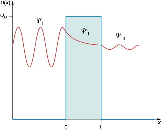
The constants A, B, F, and G in (Figure) and (Figure) may be complex. These solutions are illustrated in (Figure). In region I, there are two waves—one is incident (moving to the right) and one is reflected (moving to the left)—so none of the constants A and B in (Figure) may vanish. In region III, there is only one wave (moving to the right), which is the transmitted wave, so the constant G must be zero in (Figure), $G=0$ . We can write explicitly that the incident wave is ${\psi }_{\text{in}}\left(x\right)=A{e}^{+ikx}$ and that the reflected wave is ${\psi }_{\text{ref}}\left(x\right)=B{e}^{\text{−}ikx}$ , and that the transmitted wave is ${\psi }_{\text{tra}}\left(x\right)=F{e}^{+ikx}$ . The amplitude of the incident wave is

$|{\psi }_{\text{in}}\left(x\right){|}^{2}={\psi }_{\text{in}}^{*}\left(x\right){\psi }_{\text{in}}\left(x\right)={\left(A{e}^{+ikx}\right)}^{*}A{e}^{+ikx}={A}^{*}{e}^{\text{−}ikx}A{e}^{+ikx}={A}^{*}A=|A{|}^{2}.$

Similarly, the amplitude of the reflected wave is $|{\psi }_{\text{ref}}\left(x\right){|}^{2}=|B{|}^{2}$ and the amplitude of the transmitted wave is $|{\psi }_{\text{tra}}\left(x\right){|}^{2}=|F{|}^{2}$ . We know from the theory of waves that the square of the wave amplitude is directly proportional to the wave intensity. If we want to know how much of the incident wave tunnels through the barrier, we need to compute the square of the amplitude of the transmitted wave. The transmission probability or tunneling probability is the ratio of the transmitted intensity $\left(|F{|}^{2}\right)$ to the incident intensity $\left(|A{|}^{2}\right)$ , written as

$T\left(L,E\right)=\frac{|{\psi }_{\text{tra}}\left(x\right){|}^{2}}{|{\psi }_{\text{in}}\left(x\right){|}^{2}}=\frac{|F{|}^{2}}{|A{|}^{2}}={|\frac{F}{A}|}^{2}$

where L is the width of the barrier and E is the total energy of the particle. This is the probability an individual particle in the incident beam will tunnel through the potential barrier. Intuitively, we understand that this probability must depend on the barrier height ${U}_{0}$ .

In region II, the terms in equation (Figure) can be rearranged to

$\frac{{d}^{2}{\psi }_{\text{II}}\left(x\right)}{d{x}^{2}}={\beta }^{2}{\psi }_{\text{II}}\left(x\right)$

where ${\beta }^{2}$ is positive because ${U}_{0}>E$ and the parameter $\beta$ is a real number,

${\beta }^{2}=\frac{2m}{{\hslash }^{2}}\left({U}_{0}-E\right).$

The general solution to (Figure) is not oscillatory (unlike in the other regions) and is in the form of exponentials that describe a gradual attenuation of ${\psi }_{\text{II}}\left(x\right)$ ,

${\psi }_{\text{II}}\left(x\right)=C{e}^{\text{−}\beta x}+D{e}^{+\beta x}.$

The two types of solutions in the three regions are illustrated in (Figure).

Three types of solutions to the stationary Schrӧdinger equation for the quantum-tunneling problem: Oscillatory behavior in regions I and III where a quantum particle moves freely, and exponential-decay behavior in region II (the barrier region) where the particle moves in the potential ${U}_{0}$ .

Now we use the boundary conditions to find equations for the unknown constants. (Figure) and (Figure) are substituted into (Figure) to give

$A+B=C+D.$

(Figure) and (Figure) are substituted into (Figure) to give

$C{e}^{\text{−}\beta L}+D{e}^{+\beta L}=F{e}^{+ikL}.$

Similarly, we substitute (Figure) and (Figure) into (Figure), differentiate, and obtain

$\text{−}ik\left(A-B\right)=\beta \left(D-C\right).$

Similarly, the boundary condition (Figure) reads explicitly

$\beta \left(D{e}^{+\beta L}-C{e}^{\text{−}\beta L}\right)=\text{−}ikF{e}^{+ikL}.$

We now have four equations for five unknown constants. However, because the quantity we are after is the transmission coefficient, defined in (Figure) by the fraction F/A, the number of equations is exactly right because when we divide each of the above equations by A, we end up having only four unknown fractions: B/A, C/A, D/A, and F/A, three of which can be eliminated to find F/A. The actual algebra that leads to expression for F/A is pretty lengthy, but it can be done either by hand or with a help of computer software. The end result is

$\frac{F}{A}=\frac{{e}^{\text{−}ikL}}{\text{cosh}\phantom{\rule{0.2em}{0ex}}\left(\beta L\right)+i\left(\gamma \text{/}2\right)\text{sinh}\phantom{\rule{0.2em}{0ex}}\left(\beta L\right)}.$

In deriving (Figure), to avoid the clutter, we use the substitutions $\gamma \equiv \beta \text{/}k-k\text{/}\beta$ ,

$\text{cosh}\phantom{\rule{0.2em}{0ex}}y=\frac{{e}^{y}+{e}^{\text{−}y}}{2},\text{and}\phantom{\rule{0.2em}{0ex}}\text{sinh}\phantom{\rule{0.2em}{0ex}}y=\frac{{e}^{y}-{e}^{\text{−}y}}{2}.$

We substitute (Figure) into (Figure) and obtain the exact expression for the transmission coefficient for the barrier,

$T\left(L,E\right)=\left(\frac{F}{A}{\right)}^{*}\frac{F}{A}=\frac{{e}^{+ikL}}{\text{cosh}\phantom{\rule{0.2em}{0ex}}\left(\beta L\right)-i\left(\gamma \text{/}2\right)\text{sinh}\phantom{\rule{0.2em}{0ex}}\left(\beta L\right)}·\frac{{e}^{\text{−}ikL}}{\text{cosh}\phantom{\rule{0.2em}{0ex}}\left(\beta L\right)+i\left(\gamma \text{/}2\right)\text{sinh}\phantom{\rule{0.2em}{0ex}}\left(\beta L\right)}$

or

$T\left(L,E\right)=\frac{1}{{\text{cosh}}^{2}\left(\beta L\right)+{\left(\gamma \text{/}2\right)}^{2}{\text{sinh}}^{2}\left(\beta L\right)}$

where

${\left(\frac{\gamma }{2}\right)}^{2}=\frac{1}{4}\left(\frac{1-E\text{/}{U}_{0}}{E\text{/}{U}_{0}}+\frac{E\text{/}{U}_{0}}{1-E\text{/}{U}_{0}}-2\right).$

For a wide and high barrier that transmits poorly, (Figure) can be approximated by

$T\left(L,E\right)=16\frac{E}{{U}_{0}}\left(1-\frac{E}{{U}_{0}}\right){e}^{\text{−}2\beta L}.$

Whether it is the exact expression (Figure) or the approximate expression (Figure), we see that the tunneling effect very strongly depends on the width L of the potential barrier. In the laboratory, we can adjust both the potential height ${U}_{0}$ and the width L to design nano-devices with desirable transmission coefficients.

Transmission Coefficient Two copper nanowires are insulated by a copper oxide nano-layer that provides a 10.0-eV potential barrier. Estimate the tunneling probability between the nanowires by 7.00-eV electrons through a 5.00-nm thick oxide layer. What if the thickness of the layer were reduced to just 1.00 nm? What if the energy of electrons were increased to 9.00 eV?

Strategy Treating the insulating oxide layer as a finite-height potential barrier, we use (Figure). We identify ${U}_{0}=10.0\phantom{\rule{0.2em}{0ex}}\text{eV}$ , ${E}_{1}=7.00\phantom{\rule{0.2em}{0ex}}\text{eV}$ , ${E}_{2}=9.00\phantom{\rule{0.2em}{0ex}}\text{eV}$ , ${L}_{1}=5.00\phantom{\rule{0.2em}{0ex}}\text{nm}$ , and ${L}_{2}=1.00\phantom{\rule{0.2em}{0ex}}\text{nm}$ . We use (Figure) to compute the exponent. Also, we need the rest mass of the electron $m=511\phantom{\rule{0.2em}{0ex}}\text{keV}\text{/}{c}^{2}$ and Planck’s constant $\hslash =0.1973\text{keV}·\text{nm}\text{/}c$ . It is typical for this type of estimate to deal with very small quantities that are often not suitable for handheld calculators. To make correct estimates of orders, we make the conversion ${e}^{y}={10}^{y\text{/}\text{ln}\phantom{\rule{0.2em}{0ex}}10}$ .

Solution Constants:

$\frac{2m}{{\hslash }^{2}}=\frac{2\left(511\phantom{\rule{0.2em}{0ex}}\text{keV}\text{/}{c}^{2}\right)}{{\left(0.1973\text{keV}·\text{nm}\text{/}c\right)}^{2}}=26,254\frac{1}{\text{keV}·{\left(\text{nm)}}^{2}},$

$\beta =\sqrt{\frac{2m}{{\hslash }^{2}}\left({U}_{0}-E\right)}=\sqrt{26,254\frac{\left(10.0\phantom{\rule{0.2em}{0ex}}\text{eV}-E\right)}{\text{keV}·{\left(\text{nm)}}^{2}}}=\sqrt{26.254\left(10.0\phantom{\rule{0.2em}{0ex}}\text{eV}-E\right)\text{/}\text{eV}}\frac{1}{\text{nm}}.$

For a lower-energy electron with ${E}_{1}=7.00\phantom{\rule{0.2em}{0ex}}\text{eV}$ :

${\beta }_{1}=\sqrt{26.254\left(10.00\phantom{\rule{0.2em}{0ex}}\text{eV}-{E}_{1}\right)\text{/}\text{eV}}\frac{1}{\text{nm}}=\sqrt{26.254\left(10.00-7.00\right)}\frac{1}{\text{nm}}=\frac{8.875}{\text{nm}},$

$T\left(L,{E}_{1}\right)=16\frac{{E}_{1}}{{U}_{0}}\left(1-\frac{{E}_{1}}{{U}_{0}}\right){e}^{\text{−}2{\beta }_{1}L}=16\frac{7}{10}\left(1-\frac{7}{10}\right){e}^{\text{−}17.75\phantom{\rule{0.2em}{0ex}}L\text{/}\text{nm}}=3.36{e}^{\text{−}17.75\phantom{\rule{0.2em}{0ex}}L\text{/}\text{nm}}.$

For a higher-energy electron with ${E}_{2}=9.00\phantom{\rule{0.2em}{0ex}}\text{eV}$ :

${\beta }_{2}=\sqrt{26.254\left(10.00\phantom{\rule{0.2em}{0ex}}\text{eV}-{E}_{2}\right)\text{/}\text{eV}}\frac{1}{\text{nm}}=\sqrt{26.254\left(10.00-9.00\right)}\frac{1}{\text{nm}}=\frac{5.124}{\text{nm}},$

$T\left(L,{E}_{2}\right)=16\frac{{E}_{2}}{{U}_{0}}\left(1-\frac{{E}_{2}}{{U}_{0}}\right){e}^{\text{−}2{\beta }_{2}\phantom{\rule{0.2em}{0ex}}L}=16\frac{9}{10}\left(1-\frac{9}{10}\right){e}^{\text{−}5.12\phantom{\rule{0.2em}{0ex}}L\text{/}\text{nm}}=1.44{e}^{\text{−}5.12\phantom{\rule{0.2em}{0ex}}L\text{/}\text{nm}}.$

For a broad barrier with ${L}_{1}=5.00\phantom{\rule{0.2em}{0ex}}\text{nm}$ :

*** QuickLaTeX cannot compile formula:
T\left({L}_{1},{E}_{1}\right)=3.36{e}^{\text{−}17.75\phantom{\rule{0.2em}{0ex}}{L}_{1}\text{/}\text{nm}}=3.36{e}^{\text{−}17.75·5.00\phantom{\rule{0.2em}{0ex}}\text{nm}\text{/}\text{nm}}=3.36{e}^{-88}=3.36\left(6.2\phantom{\rule{0.2em}{0ex}}×\phantom{\rule{0.2em}{0ex}}{10}^{-39}\right)=2.1\text{%}\phantom{\rule{0.2em}{0ex}}×\phantom{\rule{0.2em}{0ex}}{10}^{-36},

*** Error message:
Unicode character − (U+2212)
leading text: ...({L}_{1},{E}_{1}\right)=3.36{e}^{\text{−}
Unicode character − (U+2212)
leading text: ...}_{1}\text{/}\text{nm}}=3.36{e}^{\text{−}
File ended while scanning use of \text@.
Emergency stop.

*** QuickLaTeX cannot compile formula:
T\left({L}_{1},{E}_{2}\right)=1.44{e}^{\text{−}5.12\phantom{\rule{0.2em}{0ex}}{L}_{1}\text{/}\text{nm}}=1.44{e}^{\text{−}5.12·5.00\phantom{\rule{0.2em}{0ex}}\text{nm}\text{/}\text{nm}}=1.44{e}^{\text{−}25.6}=1.44\left(7.62\phantom{\rule{0.2em}{0ex}}×\phantom{\rule{0.2em}{0ex}}{10}^{-12}\right)=1.1\text{%}\phantom{\rule{0.2em}{0ex}}×\phantom{\rule{0.2em}{0ex}}{10}^{-9}.

*** Error message:
Unicode character − (U+2212)
leading text: ...({L}_{1},{E}_{2}\right)=1.44{e}^{\text{−}
Unicode character − (U+2212)
leading text: ...}_{1}\text{/}\text{nm}}=1.44{e}^{\text{−}
Unicode character − (U+2212)
leading text: ...t{nm}\text{/}\text{nm}}=1.44{e}^{\text{−}
File ended while scanning use of \text@.
Emergency stop.

For a narrower barrier with ${L}_{2}=1.00\phantom{\rule{0.2em}{0ex}}\text{nm}$ :

*** QuickLaTeX cannot compile formula:
T\left({L}_{2},{E}_{1}\right)=3.36{e}^{\text{−}17.75\phantom{\rule{0.2em}{0ex}}{L}_{2}\text{/}\text{nm}}=3.36{e}^{\text{−}17.75·1.00\phantom{\rule{0.2em}{0ex}}\text{nm}\text{/}\text{nm}}=3.36{e}^{-17.75}=3.36\left(5.1\phantom{\rule{0.2em}{0ex}}×\phantom{\rule{0.2em}{0ex}}{10}^{-7}\right)=1.7\text{%}\phantom{\rule{0.2em}{0ex}}×\phantom{\rule{0.2em}{0ex}}{10}^{-4},

*** Error message:
Unicode character − (U+2212)
leading text: ...({L}_{2},{E}_{1}\right)=3.36{e}^{\text{−}
Unicode character − (U+2212)
leading text: ...}_{2}\text{/}\text{nm}}=3.36{e}^{\text{−}
File ended while scanning use of \text@.
Emergency stop.

*** QuickLaTeX cannot compile formula:
T\left({L}_{2},{E}_{2}\right)=1.44{e}^{\text{−}5.12\phantom{\rule{0.2em}{0ex}}{L}_{2}\text{/}\text{nm}}=1.44{e}^{\text{−}5.12·1.00\phantom{\rule{0.2em}{0ex}}\text{nm}\text{/}\text{nm}}=1.44{e}^{\text{−}5.12}=1.44\left(5.98\phantom{\rule{0.2em}{0ex}}×\phantom{\rule{0.2em}{0ex}}{10}^{-3}\right)=0.86\text{%}.

*** Error message:
Unicode character − (U+2212)
leading text: ...({L}_{2},{E}_{2}\right)=1.44{e}^{\text{−}
Unicode character − (U+2212)
leading text: ...}_{2}\text{/}\text{nm}}=1.44{e}^{\text{−}
Unicode character − (U+2212)
leading text: ...t{nm}\text{/}\text{nm}}=1.44{e}^{\text{−}
File ended while scanning use of \text@.
Emergency stop.

Significance We see from these estimates that the probability of tunneling is affected more by the width of the potential barrier than by the energy of an incident particle. In today’s technologies, we can manipulate individual atoms on metal surfaces to create potential barriers that are fractions of a nanometer, giving rise to measurable tunneling currents. One of many applications of this technology is the scanning tunneling microscope (STM), which we discuss later in this section.

Check Your Understanding A proton with kinetic energy 1.00 eV is incident on a square potential barrier with height 10.00 eV. If the proton is to have the same transmission probability as an electron of the same energy, what must the width of the barrier be relative to the barrier width encountered by an electron?

*** QuickLaTeX cannot compile formula:
{L}_{\text{proton}}\text{/}{L}_{\text{electron}}=\sqrt{{m}_{e}\text{/}{m}_{p}}=2.3\text{%}

*** Error message:
File ended while scanning use of \text@.
Emergency stop.

Radioactive Decay

In 1928, Gamow identified quantum tunneling as the mechanism responsible for the radioactive decay of atomic nuclei. He observed that some isotopes of thorium, uranium, and bismuth disintegrate by emitting $\text{α}$ -particles (which are doubly ionized helium atoms or, simply speaking, helium nuclei). In the process of emitting an $\text{α}$ -particle, the original nucleus is transformed into a new nucleus that has two fewer neutrons and two fewer protons than the original nucleus. The $\text{α}$ -particles emitted by one isotope have approximately the same kinetic energies. When we look at variations of these energies among isotopes of various elements, the lowest kinetic energy is about 4 MeV and the highest is about 9 MeV, so these energies are of the same order of magnitude. This is about where the similarities between various isotopes end.

When we inspect half-lives (a half-life is the time in which a radioactive sample loses half of its nuclei due to decay), different isotopes differ widely. For example, the half-life of polonium-214 is $160\phantom{\rule{0.2em}{0ex}}µ\text{s}$ and the half-life of uranium is 4.5 billion years. Gamow explained this variation by considering a ‘spherical-box’ model of the nucleus, where $\text{α}$ -particles can bounce back and forth between the walls as free particles. The confinement is provided by a strong nuclear potential at a spherical wall of the box. The thickness of this wall, however, is not infinite but finite, so in principle, a nuclear particle has a chance to escape this nuclear confinement. On the inside wall of the confining barrier is a high nuclear potential that keeps the $\text{α}$ -particle in a small confinement. But when an $\text{α}$ -particle gets out to the other side of this wall, it is subject to electrostatic Coulomb repulsion and moves away from the nucleus. This idea is illustrated in (Figure). The width L of the potential barrier that separates an $\text{α}$ -particle from the outside world depends on the particle’s kinetic energy E. This width is the distance between the point marked by the nuclear radius R and the point ${R}_{0}$ where an $\text{α}$ -particle emerges on the other side of the barrier, $L={R}_{0}-R$ . At the distance ${R}_{0}$ , its kinetic energy must at least match the electrostatic energy of repulsion, $E={\left(4\pi {\epsilon }_{0}\right)}^{-1}Z{e}^{2}\text{/}{R}_{0}$ (where $+Ze$ is the charge of the nucleus). In this way we can estimate the width of the nuclear barrier,

$L=\frac{{e}^{2}}{4\pi {\epsilon }_{0}}\phantom{\rule{0.2em}{0ex}}\frac{Z}{E}-R.$

We see from this estimate that the higher the energy of $\text{α}$ -particle, the narrower the width of the barrier that it is to tunnel through. We also know that the width of the potential barrier is the most important parameter in tunneling probability. Thus, highly energetic $\text{α}$ -particles have a good chance to escape the nucleus, and, for such nuclei, the nuclear disintegration half-life is short. Notice that this process is highly nonlinear, meaning a small increase in the $\text{α}$ -particle energy has a disproportionately large enhancing effect on the tunneling probability and, consequently, on shortening the half-life. This explains why the half-life of polonium that emits 8-MeV $\text{α}$ -particles is only hundreds of milliseconds and the half-life of uranium that emits 4-MeV $\text{α}$ -particles is billions of years.

The potential energy barrier for an $\text{α}$ -particle bound in the nucleus: To escape from the nucleus, an $\text{α}$ -particle with energy E must tunnel across the barrier from distance R to distance ${R}_{0}$ away from the center.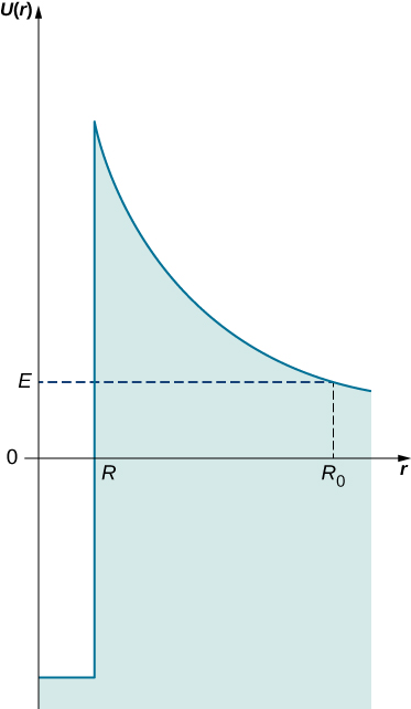

The potential U of r is plotted as a function of r. For r less than R, U of r is constant and negative. At r = R, the potential rises vertically to some maximum positive value, then decays toward zero. The area under the curve is shaded. U of r equals E at r equal to R sub 0. A horizontal dashed line at E=E and a vertical dashed line at r=R sub 0 are shown.

Field Emission

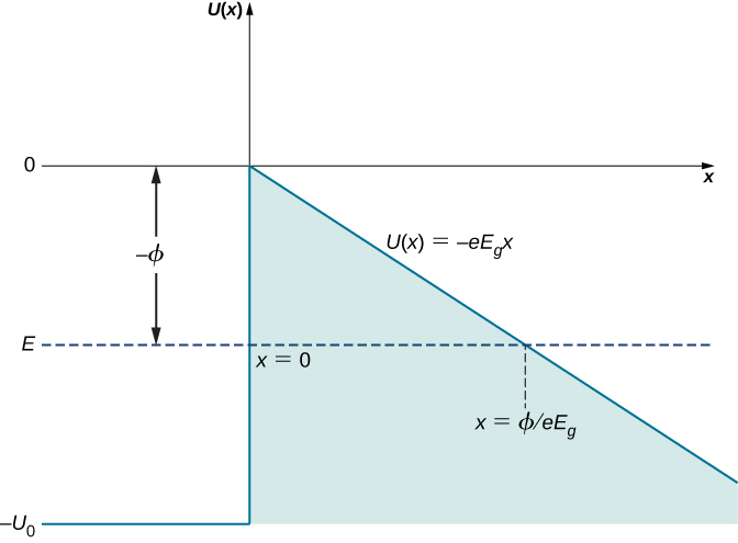
Field emission is a process of emitting electrons from conducting surfaces due to a strong external electric field that is applied in the direction normal to the surface ((Figure)). As we know from our study of electric fields in earlier chapters, an applied external electric field causes the electrons in a conductor to move to its surface and stay there as long as the present external field is not excessively strong. In this situation, we have a constant electric potential throughout the inside of the conductor, including its surface. In the language of potential energy, we say that an electron inside the conductor has a constant potential energy $U\left(x\right)=\text{−}{U}_{0}$ (here, the x means inside the conductor). In the situation represented in (Figure), where the external electric field is uniform and has magnitude ${E}_{g}$ , if an electron happens to be outside the conductor at a distance x away from its surface, its potential energy would have to be $U\left(x\right)=\text{−}e{E}_{g}x$ (here, x denotes distance to the surface). Taking the origin at the surface, so that $x=0$ is the location of the surface, we can represent the potential energy of conduction electrons in a metal as the potential energy barrier shown in (Figure). In the absence of the external field, the potential energy becomes a step barrier defined by $U\left(x\le 0\right)=\text{−}{U}_{0}$ and by $U\left(x>0\right)=0$ .

A normal-direction external electric field at the surface of a conductor: In a strong field, the electrons on a conducting surface may get detached from it and accelerate against the external electric field away from the surface.

The potential U of r is plotted as a function of r. For r less than R, U of r is constant and negative. At r = R, the potential rises vertically to some maximum positive value, then decays toward zero. The area under the curve is shaded. U of r equals E at r equal to R sub 0. A horizontal dashed line at E=E and a vertical dashed line at r=R sub 0 are shown.

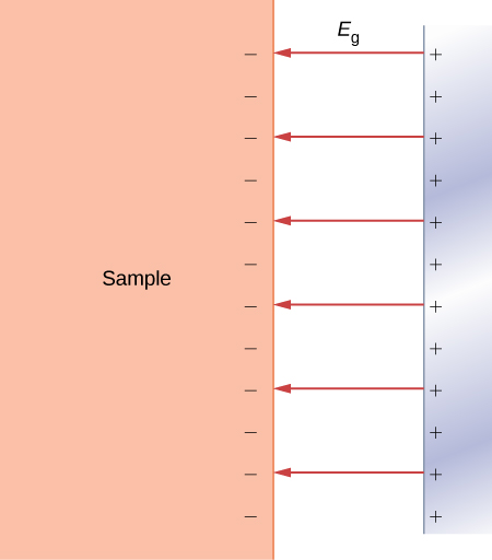
The potential energy barrier at the surface of a metallic conductor in the presence of an external uniform electric field ${E}_{g}$ normal to the surface: It becomes a step-function barrier when the external field is removed. The work function of the metal is indicated by $\varphi .$

When an external electric field is strong, conduction electrons at the surface may get detached from it and accelerate along electric field lines in a direction antiparallel to the external field, away from the surface. In short, conduction electrons may escape from the surface. The field emission can be understood as the quantum tunneling of conduction electrons through the potential barrier at the conductor’s surface. The physical principle at work here is very similar to the mechanism of $\text{α}$ -emission from a radioactive nucleus.

Suppose a conduction electron has a kinetic energy E (the average kinetic energy of an electron in a metal is the work function $\varphi$ for the metal and can be measured, as discussed for the photoelectric effect in Photons and Matter Waves), and an external electric field can be locally approximated by a uniform electric field of strength ${E}_{g}$ . The width L of the potential barrier that the electron must cross is the distance from the conductor’s surface to the point outside the surface where its kinetic energy matches the value of its potential energy in the external field. In (Figure), this distance is measured along the dashed horizontal line $U\left(x\right)=E$ from $x=0$ to the intercept with $U\left(x\right)=\text{−}e{E}_{g}x$ , so the barrier width is

$L=\frac{{e}^{-1}E}{{E}_{g}}=\frac{{e}^{-1}\varphi }{{E}_{g}}.$

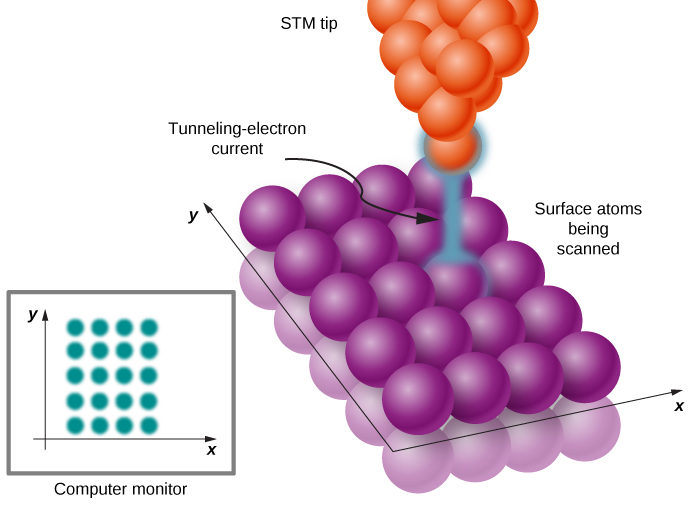
We see that L is inversely proportional to the strength ${E}_{g}$ of an external field. When we increase the strength of the external field, the potential barrier outside the conductor becomes steeper and its width decreases for an electron with a given kinetic energy. In turn, the probability that an electron will tunnel across the barrier (conductor surface) becomes exponentially larger. The electrons that emerge on the other side of this barrier form a current (tunneling-electron current) that can be detected above the surface. The tunneling-electron current is proportional to the tunneling probability. The tunneling probability depends nonlinearly on the barrier width L, and L can be changed by adjusting ${E}_{g}$ . Therefore, the tunneling-electron current can be tuned by adjusting the strength of an external electric field at the surface. When the strength of an external electric field is constant, the tunneling-electron current has different values at different elevations L above the surface.

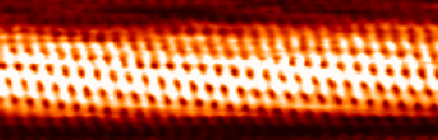
The quantum tunneling phenomenon at metallic surfaces, which we have just described, is the physical principle behind the operation of the scanning tunneling microscope (STM), invented in 1981 by Gerd Binnig and Heinrich Rohrer. The STM device consists of a scanning tip (a needle, usually made of tungsten, platinum-iridium, or gold); a piezoelectric device that controls the tip’s elevation in a typical range of 0.4 to 0.7 nm above the surface to be scanned; some device that controls the motion of the tip along the surface; and a computer to display images. While the sample is kept at a suitable voltage bias, the scanning tip moves along the surface ((Figure)), and the tunneling-electron current between the tip and the surface is registered at each position. The amount of the current depends on the probability of electron tunneling from the surface to the tip, which, in turn, depends on the elevation of the tip above the surface. Hence, at each tip position, the distance from the tip to the surface is measured by measuring how many electrons tunnel out from the surface to the tip. This method can give an unprecedented resolution of about 0.001 nm, which is about 1% of the average diameter of an atom. In this way, we can see individual atoms on the surface, as in the image of a carbon nanotube in (Figure).

In STM, a surface at a constant potential is being scanned by a narrow tip moving along the surface. When the STM tip moves close to surface atoms, electrons can tunnel from the surface to the tip. This tunneling-electron current is continually monitored while the tip is in motion. The amount of current at location (x,y) gives information about the elevation of the tip above the surface at this location. In this way, a detailed topographical map of the surface is created and displayed on a computer monitor.

An STM image of a carbon nanotube: Atomic-scale resolution allows us to see individual atoms on the surface. STM images are in gray scale, and coloring is added to bring up details to the human eye. (credit: Taner Yildirim, NIST)

An STM image of a carbon nanotube showing the atoms as red points in a grid like pattern.

Resonant Quantum Tunneling

Quantum tunneling has numerous applications in semiconductor devices such as electronic circuit components or integrated circuits that are designed at nanoscales; hence, the term ‘nanotechnology.’ For example, a diode (an electric-circuit element that causes an electron current in one direction to be different from the current in the opposite direction, when the polarity of the bias voltage is reversed) can be realized by a tunneling junction between two different types of semiconducting materials. In such a tunnel diode, electrons tunnel through a single potential barrier at a contact between two different semiconductors. At the junction, tunneling-electron current changes nonlinearly with the applied potential difference across the junction and may rapidly decrease as the bias voltage is increased. This is unlike the Ohm’s law behavior that we are familiar with in household circuits. This kind of rapid behavior (caused by quantum tunneling) is desirable in high-speed electronic devices.

Another kind of electronic nano-device utilizes resonant tunneling of electrons through potential barriers that occur in quantum dots. A quantum dot is a small region of a semiconductor nanocrystal that is grown, for example, in a silicon or aluminum arsenide crystal. (Figure)(a) shows a quantum dot of gallium arsenide embedded in an aluminum arsenide wafer. The quantum-dot region acts as a potential well of a finite height (shown in (Figure)(b)) that has two finite-height potential barriers at dot boundaries. Similarly, as for a quantum particle in a box (that is, an infinite potential well), lower-lying energies of a quantum particle trapped in a finite-height potential well are quantized. The difference between the box and the well potentials is that a quantum particle in a box has an infinite number of quantized energies and is trapped in the box indefinitely, whereas a quantum particle trapped in a potential well has a finite number of quantized energy levels and can tunnel through potential barriers at well boundaries to the outside of the well. Thus, a quantum dot of gallium arsenide sitting in aluminum arsenide is a potential well where low-lying energies of an electron are quantized, indicated as ${E}_{\text{dot}}$ in part (b) in the figure. When the energy ${E}_{\text{electron}}$ of an electron in the outside region of the dot does not match its energy ${E}_{\text{dot}}$ that it would have in the dot, the electron does not tunnel through the region of the dot and there is no current through such a circuit element, even if it were kept at an electric voltage difference (bias). However, when this voltage bias is changed in such a way that one of the barriers is lowered, so that ${E}_{\text{dot}}$ and ${E}_{\text{electron}}$ become aligned, as seen in part (c) of the figure, an electron current flows through the dot. When the voltage bias is now increased, this alignment is lost and the current stops flowing. When the voltage bias is increased further, the electron tunneling becomes improbable until the bias voltage reaches a value for which the outside electron energy matches the next electron energy level in the dot. The word ‘resonance’ in the device name means that the tunneling-electron current occurs only when a selected energy level is matched by tuning an applied voltage bias, such as in the operation mechanism of the resonant-tunneling diode just described. Resonant-tunneling diodes are used as super-fast nano-switches.

Resonant-tunneling diode: (a) A quantum dot of gallium arsenide embedded in aluminum arsenide. (b) Potential well consisting of two potential barriers of a quantum dot with no voltage bias. Electron energies ${E}_{\text{electron}}$ in aluminum arsenide are not aligned with their energy levels ${E}_{\text{dot}}$ in the quantum dot, so electrons do not tunnel through the dot. (c) Potential well of the dot with a voltage bias across the device. A suitably tuned voltage difference distorts the well so that electron-energy levels in the dot are aligned with their energies in aluminum arsenide, causing the electrons to tunnel through the dot.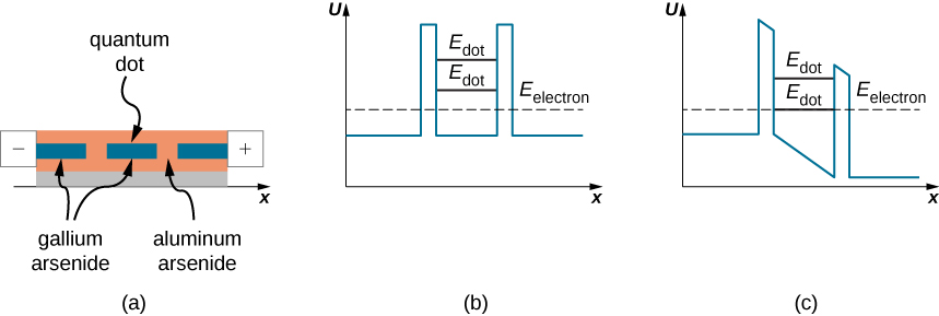

Summary

A quantum particle that is incident on a potential barrier of a finite width and height may cross the barrier and appear on its other side. This phenomenon is called ‘quantum tunneling.’ It does not have a classical analog.
To find the probability of quantum tunneling, we assume the energy of an incident particle and solve the stationary Schrӧdinger equation to find wave functions inside and outside the barrier. The tunneling probability is a ratio of squared amplitudes of the wave past the barrier to the incident wave.
The tunneling probability depends on the energy of the incident particle relative to the height of the barrier and on the width of the barrier. It is strongly affected by the width of the barrier in a nonlinear, exponential way so that a small change in the barrier width causes a disproportionately large change in the transmission probability.
Quantum-tunneling phenomena govern radioactive nuclear decays. They are utilized in many modern technologies such as STM and nano-electronics. STM allows us to see individual atoms on metal surfaces. Electron-tunneling devices have revolutionized electronics and allow us to build fast electronic devices of miniature sizes.

Key Equations

Normalization condition in one dimension	$P\left(x=\text{−}\infty ,\text{+}\infty \right)=\underset{\text{−}\infty }{\overset{\infty }{\int }}\|\text{Ψ}\left(x,t\right){\|}^{2}dx=1$
Probability of finding a particle in a narrow interval of position in one dimension $\left(x,x+dx\right)$	$P\left(x,x+dx\right)={\text{Ψ}}^{*}\left(x,t\right)\text{Ψ}\left(x,t\right)dx$
Expectation value of position in one dimension	$〈x〉=\underset{\text{−}\infty }{\overset{\infty }{\int }}{\text{Ψ}}^{*}\left(x,t\right)x\text{Ψ}\left(x,t\right)dx$
Heisenberg’s position-momentum uncertainty principle	$\text{Δ}x\text{Δ}p\ge \frac{\hslash }{2}$
Heisenberg’s energy-time uncertainty principle	$\text{Δ}E\text{Δ}t\ge \frac{\hslash }{2}$
Schrӧdinger’s time-dependent equation	$-\frac{{\hslash }^{2}}{2m}\phantom{\rule{0.2em}{0ex}}\frac{{\partial }^{2}\text{Ψ}\left(x,t\right)}{\partial {x}^{2}}+U\left(x,t\right)\text{Ψ}\left(x,t\right)=i\hslash \frac{{\partial }^{2}\text{Ψ}\left(x,t\right)}{\partial t}$
General form of the wave function for a time-independent potential in one dimension	$\text{Ψ}\left(x,t\right)=\psi \left(x\right){e}^{\text{−}i\omega t}$
Schrӧdinger’s time-independent equation	$-\frac{{\hslash }^{2}}{2m}\phantom{\rule{0.2em}{0ex}}\frac{{d}^{2}\psi \left(x\right)}{d{x}^{2}}+U\left(x\right)\psi \left(x\right)=E\psi \left(x\right)$
Schrӧdinger’s equation (free particle)	$-\frac{{\hslash }^{2}}{2m}\phantom{\rule{0.2em}{0ex}}\frac{{\partial }^{2}\psi \left(x\right)}{\partial {x}^{2}}=E\psi \left(x\right)$
Allowed energies (particle in box of length L)	${E}_{n}={n}^{2}\frac{{\pi }^{2}{\hslash }^{2}}{2m{L}^{2}},n=1,2,3,...$
Stationary states (particle in a box of length L)	${\psi }_{n}\left(x\right)=\sqrt{\frac{2}{L}}\phantom{\rule{0.2em}{0ex}}\text{sin}\phantom{\rule{0.2em}{0ex}}\frac{n\pi x}{L},n=1,2,3,...$
Potential-energy function of a harmonic oscillator	$U\left(x\right)=\frac{1}{2}m{\omega }^{2}{x}^{2}$
Stationary Schrӧdinger equation	$-\frac{\hslash }{2m}\phantom{\rule{0.2em}{0ex}}\frac{{d}^{2}\psi \left(x\right)}{d{x}^{2}}+\frac{1}{2}m{\omega }^{2}{x}^{2}\psi \left(x\right)=E\psi \left(x\right)$
The energy spectrum	${E}_{n}=\left(n+\frac{1}{2}\right)\hslash \omega ,n=0,1,2,3,...$
The energy wave functions	${\psi }_{n}\left(x\right)={N}_{n}{e}^{\text{−}{\beta }^{2}{x}^{2}\text{/}2}{H}_{n}\left(\beta x\right),n=0,1,2,3,...$
Potential barrier	$U\left(x\right)=\left\{\begin{array}{cc}\hfill 0,& \text{when}\phantom{\rule{0.2em}{0ex}}x<0\hfill \\ \hfill {U}_{0},& \text{when}\phantom{\rule{0.2em}{0ex}}0\le x\le L\hfill \\ \hfill 0,& \text{when}\phantom{\rule{0.2em}{0ex}}x>L\hfill \end{array}$
Definition of the transmission coefficient	$T\left(L,E\right)=\frac{\|{\psi }_{\text{tra}}\left(x\right){\|}^{2}}{\|{\psi }_{\text{in}}\left(x\right){\|}^{2}}$
A parameter in the transmission coefficient	${\beta }^{2}=\frac{2m}{{\hslash }^{2}}\left({U}_{0}-E\right)$
Transmission coefficient, exact	$T\left(L,E\right)=\frac{1}{{\text{cosh}}^{2}\beta L+{\left(\gamma \text{/}2\right)}^{2}{\text{sinh}}^{2}\beta L}$
Transmission coefficient, approximate	$T\left(L,E\right)=16\frac{E}{{U}_{0}}\left(1-\frac{E}{{U}_{0}}\right){e}^{\text{−}2\beta \phantom{\rule{0.2em}{0ex}}L}$

Conceptual Questions

When an electron and a proton of the same kinetic energy encounter a potential barrier of the same height and width, which one of them will tunnel through the barrier more easily? Why?

What decreases the tunneling probability most: doubling the barrier width or halving the kinetic energy of the incident particle?

doubling the barrier width

Explain the difference between a box-potential and a potential of a quantum dot.

Can a quantum particle ‘escape’ from an infinite potential well like that in a box? Why? Why not?

No, the restoring force on the particle at the walls of an infinite square well is infinity.

A tunnel diode and a resonant-tunneling diode both utilize the same physics principle of quantum tunneling. In what important way are they different?

Problems

Show that the wave function in (a) (Figure) satisfies (Figure), and (b) (Figure) satisfies (Figure).

A complex function of the form, $A{e}^{i\varphi }$ , satisfies Schrӧdinger’s time-independent equation. The operators for kinetic and total energy are linear, so any linear combination of such wave functions is also a valid solution to Schrӧdinger’s equation. Therefore, we conclude that (Figure) satisfies (Figure), and (Figure) satisfies (Figure).

A 6.0-eV electron impacts on a barrier with height 11.0 eV. Find the probability of the electron to tunnel through the barrier if the barrier width is (a) 0.80 nm and (b) 0.40 nm.

A 5.0-eV electron impacts on a barrier of with 0.60 nm. Find the probability of the electron to tunnel through the barrier if the barrier height is (a) 7.0 eV; (b) 9.0 eV; and (c) 13.0 eV.

a. 4.21%; b. 0.84%; c. 0.06%

A 12.0-eV electron encounters a barrier of height 15.0 eV. If the probability of the electron tunneling through the barrier is 2.5 %, find its width.

A quantum particle with initial kinetic energy 32.0 eV encounters a square barrier with height 41.0 eV and width 0.25 nm. Find probability that the particle tunnels through this barrier if the particle is (a) an electron and, (b) a proton.

a. 0.13%; b. close to 0%

A simple model of a radioactive nuclear decay assumes that $\text{α}$ -particles are trapped inside a well of nuclear potential that walls are the barriers of a finite width 2.0 fm and height 30.0 MeV. Find the tunneling probability across the potential barrier of the wall for $\text{α}$ -particles having kinetic energy (a) 29.0 MeV and (b) 20.0 MeV. The mass of the $\text{α}$ -particle is $m=6.64\phantom{\rule{0.2em}{0ex}}×\phantom{\rule{0.2em}{0ex}}{10}^{-27}\phantom{\rule{0.2em}{0ex}}\text{kg}$ .

A muon, a quantum particle with a mass approximately 200 times that of an electron, is incident on a potential barrier of height 10.0 eV. The kinetic energy of the impacting muon is 5.5 eV and only about 0.10% of the squared amplitude of its incoming wave function filters through the barrier. What is the barrier’s width?

0.38 nm

A grain of sand with mass 1.0 mg and kinetic energy 1.0 J is incident on a potential energy barrier with height 1.000001 J and width 2500 nm. How many grains of sand have to fall on this barrier before, on the average, one passes through?

Additional Problems

Show that if the uncertainty in the position of a particle is on the order of its de Broglie’s wavelength, then the uncertainty in its momentum is on the order of the value of its momentum.

proof

The mass of a $\rho$ -meson is measured to be $770\phantom{\rule{0.2em}{0ex}}\text{MeV}\text{/}{c}^{2}$ with an uncertainty of $100\phantom{\rule{0.2em}{0ex}}\text{MeV}\text{/}{c}^{2}$ . Estimate the lifetime of this meson.

A particle of mass m is confined to a box of width L. If the particle is in the first excited state, what are the probabilities of finding the particle in a region of width 0.020 L around the given point x: (a) $x=0.25L$ ; (b) $x=0.40L$ ; (c) $x=0.75L$ ; and (d) $x=0.90L$ .

a. 4.0 %; b. 1.4 %; c. 4.0%; d. 1.4%

A particle in a box [0;L] is in the third excited state. What are its most probable positions?

A 0.20-kg billiard ball bounces back and forth without losing its energy between the cushions of a 1.5 m long table. (a) If the ball is in its ground state, how many years does it need to get from one cushion to the other? You may compare this time interval to the age of the universe. (b) How much energy is required to make the ball go from its ground state to its first excited state? Compare it with the kinetic energy of the ball moving at 2.0 m/s.

a. $t=m{L}^{2}\text{/}h=2.15\phantom{\rule{0.2em}{0ex}}×\phantom{\rule{0.2em}{0ex}}{10}^{26}\text{years}$ ; b. ${E}_{1}=1.46\phantom{\rule{0.2em}{0ex}}×\phantom{\rule{0.2em}{0ex}}{10}^{-66}\text{J,}K=0.4\phantom{\rule{0.2em}{0ex}}\text{J}$

Find the expectation value of the position squared when the particle in the box is in its third excited state and the length of the box is L.

Consider an infinite square well with wall boundaries $x=0$ and $x=L.$ Show that the function $\psi \left(x\right)=A\phantom{\rule{0.2em}{0ex}}\text{sin}\phantom{\rule{0.2em}{0ex}}kx$ is the solution to the stationary Schrӧdinger equation for the particle in a box only if $k=\sqrt{2mE}\text{/}\hslash .$ Explain why this is an acceptable wave function only if k is an integer multiple of $\pi \text{/}L.$

proof

Consider an infinite square well with wall boundaries $x=0$ and $x=L.$ Explain why the function $\psi \left(x\right)=A\phantom{\rule{0.2em}{0ex}}\text{cos}\phantom{\rule{0.2em}{0ex}}kx$ is not a solution to the stationary Schrӧdinger equation for the particle in a box.

Atoms in a crystal lattice vibrate in simple harmonic motion. Assuming a lattice atom has a mass of $9.4\phantom{\rule{0.2em}{0ex}}×\phantom{\rule{0.2em}{0ex}}{10}^{-26}\phantom{\rule{0.2em}{0ex}}\text{kg}$ , what is the force constant of the lattice if a lattice atom makes a transition from the ground state to first excited state when it absorbs a $\text{525-}µ\text{m}$ photon?

1.2 N/m

A diatomic molecule behaves like a quantum harmonic oscillator with the force constant 12.0 N/m and mass $5.60\phantom{\rule{0.2em}{0ex}}×\phantom{\rule{0.2em}{0ex}}{10}^{-26}\phantom{\rule{0.2em}{0ex}}\text{kg}$ . (a) What is the wavelength of the emitted photon when the molecule makes the transition from the third excited state to the second excited state? (b) Find the ground state energy of vibrations for this diatomic molecule.

An electron with kinetic energy 2.0 MeV encounters a potential energy barrier of height 16.0 MeV and width 2.00 nm. What is the probability that the electron emerges on the other side of the barrier?

0

A beam of mono-energetic protons with energy 2.0 MeV falls on a potential energy barrier of height 20.0 MeV and of width 1.5 fm. What percentage of the beam is transmitted through the barrier?

Challenge Problems

An electron in a long, organic molecule used in a dye laser behaves approximately like a quantum particle in a box with width 4.18 nm. Find the emitted photon when the electron makes a transition from the first excited state to the ground state and from the second excited state to the first excited state.

$19.2\phantom{\rule{0.2em}{0ex}}µ\text{m;}\phantom{\rule{0.2em}{0ex}}11.5\phantom{\rule{0.2em}{0ex}}µ\text{m}$

In STM, an elevation of the tip above the surface being scanned can be determined with a great precision, because the tunneling-electron current between surface atoms and the atoms of the tip is extremely sensitive to the variation of the separation gap between them from point to point along the surface. Assuming that the tunneling-electron current is in direct proportion to the tunneling probability and that the tunneling probability is to a good approximation expressed by the exponential function ${e}^{-2\beta \phantom{\rule{0.2em}{0ex}}L}$ with $\beta =10.0\text{/nm}$ , determine the ratio of the tunneling current when the tip is 0.500 nm above the surface to the current when the tip is 0.515 nm above the surface.

If STM is to detect surface features with local heights of about 0.00200 nm, what percent change in tunneling-electron current must the STM electronics be able to detect? Assume that the tunneling-electron current has characteristics given in the preceding problem.

3.92%

Use Heisenberg’s uncertainty principle to estimate the ground state energy of a particle oscillating on an spring with angular frequency, $\omega =\sqrt{k\text{/}m}$ , where k is the spring constant and m is the mass.

Suppose an infinite square well extends from $\text{−}L\text{/}2$ to $+L\text{/}2$ . Solve the time-independent Schrӧdinger’s equation to find the allowed energies and stationary states of a particle with mass m that is confined to this well. Then show that these solutions can be obtained by making the coordinate transformation $x\text{′}=x-L\text{/}2$ for the solutions obtained for the well extending between 0 and L.

proof

A particle of mass m confined to a box of width L is in its first excited state ${\psi }_{2}\left(x\right)$ . (a) Find its average position (which is the expectation value of the position). (b) Where is the particle most likely to be found?

Glossary

field emission: electron emission from conductor surfaces when a strong external electric field is applied in normal direction to conductor’s surface

nanotechnology: technology that is based on manipulation of nanostructures such as molecules or individual atoms to produce nano-devices such as integrated circuits

potential barrier: potential function that rises and falls with increasing values of position

quantum dot: small region of a semiconductor nanocrystal embedded in another semiconductor nanocrystal, acting as a potential well for electrons

quantum tunneling: phenomenon where particles penetrate through a potential energy barrier with a height greater than the total energy of the particles

resonant tunneling: tunneling of electrons through a finite-height potential well that occurs only when electron energies match an energy level in the well, occurs in quantum dots

resonant-tunneling diode: quantum dot with an applied voltage bias across it

scanning tunneling microscope (STM): device that utilizes quantum-tunneling phenomenon at metallic surfaces to obtain images of nanoscale structures

transmission probability: also called tunneling probability, the probability that a particle will tunnel through a potential barrier

tunnel diode: electron tunneling-junction between two different semiconductors

tunneling probability: also called transmission probability, the probability that a particle will tunnel through a potential barrier

License

Icon for the Creative Commons Attribution 4.0 International License

The Quantum Tunneling of Particles through Potential Barriers Copyright © by Samuel J. Ling; Jeff Sanny; and William Moebs is licensed under a Creative Commons Attribution 4.0 International License, except where otherwise noted.

Learning Objectives

Tunneling and Potential Energy

Tunneling and the Wave Function

Radioactive Decay

Field Emission

Resonant Quantum Tunneling

Summary

Key Equations

Conceptual Questions

Problems

Additional Problems

Challenge Problems

Glossary

License

Share This Book