The Compton Effect

Momentum of a Photon

Unlike a particle of matter that is characterized by its rest mass a photon is massless. In a vacuum, unlike a particle of matter that may vary its speed but cannot reach the speed of light, a photon travels at only one speed, which is exactly the speed of light. From the point of view of Newtonian classical mechanics, these two characteristics imply that a photon should not exist at all. For example, how can we find the linear momentum or kinetic energy of a body whose mass is zero? This apparent paradox vanishes if we describe a photon as a relativistic particle. According to the theory of special relativity, any particle in nature obeys the relativistic energy equation

This relation can also be applied to a photon. In (Figure), E is the total energy of a particle, p is its linear momentum, and is its rest mass. For a photon, we simply set in this equation. This leads to the expression for the momentum of a photon

Here the photon’s energy is the same as that of a light quantum of frequency f, which we introduced to explain the photoelectric effect:

The wave relation that connects frequency f with wavelength and speed c also holds for photons:

Therefore, a photon can be equivalently characterized by either its energy and wavelength, or its frequency and momentum. (Figure) and (Figure) can be combined into the explicit relation between a photon’s momentum and its wavelength:

Notice that this equation gives us only the magnitude of the photon’s momentum and contains no information about the direction in which the photon is moving. To include the direction, it is customary to write the photon’s momentum as a vector:

In (Figure), is the reduced Planck’s constant (pronounced “h-bar”), which is just Planck’s constant divided by the factor Vector is called the “wave vector” or propagation vector (the direction in which a photon is moving). The propagation vector shows the direction of the photon’s linear momentum vector. The magnitude of the wave vector is and is called the wave number. Notice that this equation does not introduce any new physics. We can verify that the magnitude of the vector in (Figure) is the same as that given by (Figure).

The Compton Effect

The Compton effect is the term used for an unusual result observed when X-rays are scattered on some materials. By classical theory, when an electromagnetic wave is scattered off atoms, the wavelength of the scattered radiation is expected to be the same as the wavelength of the incident radiation. Contrary to this prediction of classical physics, observations show that when X-rays are scattered off some materials, such as graphite, the scattered X-rays have different wavelengths from the wavelength of the incident X-rays. This classically unexplainable phenomenon was studied experimentally by Arthur H. Compton and his collaborators, and Compton gave its explanation in 1923.

To explain the shift in wavelengths measured in the experiment, Compton used Einstein’s idea of light as a particle. The Compton effect has a very important place in the history of physics because it shows that electromagnetic radiation cannot be explained as a purely wave phenomenon. The explanation of the Compton effect gave a convincing argument to the physics community that electromagnetic waves can indeed behave like a stream of photons, which placed the concept of a photon on firm ground.

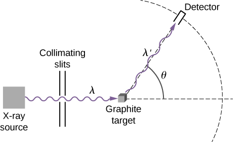
The schematics of Compton’s experimental setup are shown in (Figure). The idea of the experiment is straightforward: Monochromatic X-rays with wavelength are incident on a sample of graphite (the “target”), where they interact with atoms inside the sample; they later emerge as scattered X-rays with wavelength A detector placed behind the target can measure the intensity of radiation scattered in any direction with respect to the direction of the incident X-ray beam. This scattering angle, is the angle between the direction of the scattered beam and the direction of the incident beam. In this experiment, we know the intensity and the wavelength of the incoming (incident) beam; and for a given scattering angle we measure the intensity and the wavelength of the outgoing (scattered) beam. Typical results of these measurements are shown in (Figure), where the x-axis is the wavelength of the scattered X-rays and the y-axis is the intensity of the scattered X-rays, measured for different scattering angles (indicated on the graphs). For all scattering angles (except for we measure two intensity peaks. One peak is located at the wavelength which is the wavelength of the incident beam. The other peak is located at some other wavelength, The two peaks are separated by which depends on the scattering angle of the outgoing beam (in the direction of observation). The separation is called the Compton shift.

Experimental data show the Compton effect for X-rays scattering off graphite at various angles: The intensity of the scattered beam has two peaks. One peak appears at the wavelength of the incident radiation and the second peak appears at wavelength The separation between the peaks depends on the scattering angle which is the angular position of the detector in (Figure). The experimental data in this figure are plotted in arbitrary units so that the height of the profile reflects the intensity of the scattered beam above background noise.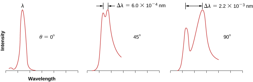

Compton Shift

As given by Compton, the explanation of the Compton shift is that in the target material, graphite, valence electrons are loosely bound in the atoms and behave like free electrons. Compton assumed that the incident X-ray radiation is a stream of photons. An incoming photon in this stream collides with a valence electron in the graphite target. In the course of this collision, the incoming photon transfers some part of its energy and momentum to the target electron and leaves the scene as a scattered photon. This model explains in qualitative terms why the scattered radiation has a longer wavelength than the incident radiation. Put simply, a photon that has lost some of its energy emerges as a photon with a lower frequency, or equivalently, with a longer wavelength. To show that his model was correct, Compton used it to derive the expression for the Compton shift. In his derivation, he assumed that both photon and electron are relativistic particles and that the collision obeys two commonsense principles: (1) the conservation of linear momentum and (2) the conservation of total relativistic energy.

In the following derivation of the Compton shift, and denote the energy and momentum, respectively, of an incident photon with frequency f. The photon collides with a relativistic electron at rest, which means that immediately before the collision, the electron’s energy is entirely its rest mass energy, Immediately after the collision, the electron has energy E and momentum both of which satisfy (Figure). Immediately after the collision, the outgoing photon has energy momentum and frequency The direction of the incident photon is horizontal from left to right, and the direction of the outgoing photon is at the angle as illustrated in (Figure). The scattering angle is the angle between the momentum vectors and and we can write their scalar product:

Following Compton’s argument, we assume that the colliding photon and electron form an isolated system. This assumption is valid for weakly bound electrons that, to a good approximation, can be treated as free particles. Our first equation is the conservation of energy for the photon-electron system:

The left side of this equation is the energy of the system at the instant immediately before the collision, and the right side of the equation is the energy of the system at the instant immediately after the collision. Our second equation is the conservation of linear momentum for the photon–electron system where the electron is at rest at the instant immediately before the collision:

The left side of this equation is the momentum of the system right before the collision, and the right side of the equation is the momentum of the system right after collision. The entire physics of Compton scattering is contained in these three preceding equations––the remaining part is algebra. At this point, we could jump to the concluding formula for the Compton shift, but it is beneficial to highlight the main algebraic steps that lead to Compton’s formula, which we give here as follows.

We start with rearranging the terms in (Figure) and squaring it:

In the next step, we substitute (Figure) for simplify, and divide both sides by to obtain

Now we can use (Figure) to express this form of the energy equation in terms of momenta. The result is

To eliminate we turn to the momentum equation (Figure), rearrange its terms, and square it to obtain

The product of the momentum vectors is given by (Figure). When we substitute this result for in (Figure), we obtain the energy equation that contains the scattering angle

With further algebra, this result can be simplified to

Now recall (Figure) and write: and When these relations are substituted into (Figure), we obtain the relation for the Compton shift:

The factor is called the Compton wavelength of the electron:

Denoting the shift as the concluding result can be rewritten as

This formula for the Compton shift describes outstandingly well the experimental results shown in (Figure). Scattering data measured for molybdenum, graphite, calcite, and many other target materials are in accord with this theoretical result. The nonshifted peak shown in (Figure) is due to photon collisions with tightly bound inner electrons in the target material. Photons that collide with the inner electrons of the target atoms in fact collide with the entire atom. In this extreme case, the rest mass in (Figure) must be changed to the rest mass of the atom. This type of shift is four orders of magnitude smaller than the shift caused by collisions with electrons and is so small that it can be neglected.

Compton scattering is an example of inelastic scattering, in which the scattered radiation has a longer wavelength than the wavelength of the incident radiation. In today’s usage, the term “Compton scattering” is used for the inelastic scattering of photons by free, charged particles. In Compton scattering, treating photons as particles with momenta that can be transferred to charged particles provides the theoretical background to explain the wavelength shifts measured in experiments; this is the evidence that radiation consists of photons.

Example

Compton Scattering

An incident 71-pm X-ray is incident on a calcite target. Find the wavelength of the X-ray scattered at a angle. What is the largest shift that can be expected in this experiment?

Strategy To find the wavelength of the scattered X-ray, first we must find the Compton shift for the given scattering angle, We use (Figure). Then we add this shift to the incident wavelength to obtain the scattered wavelength. The largest Compton shift occurs at the angle when has the largest value, which is for the angle

Solution The shift at is

This gives the scattered wavelength:

The largest shift is

Significance

The largest shift in wavelength is detected for the backscattered radiation; however, most of the photons from the incident beam pass through the target and only a small fraction of photons gets backscattered (typically, less than 5%). Therefore, these measurements require highly sensitive detectors.