Free Electron Model of Metals

Samuel J. Ling; Jeff Sanny; William Moebs

Condensed Matter Physics

Free Electron Model of Metals

Samuel J. Ling; Jeff Sanny; and William Moebs

Learning Objectives

By the end of this section, you will be able to:

Describe the classical free electron model of metals in terms of the concept electron number density
Explain the quantum free-electron model of metals in terms of Pauli’s exclusion principle
Calculate the energy levels and energy-level spacing of a free electron in a metal

Metals, such as copper and aluminum, are held together by bonds that are very different from those of molecules. Rather than sharing and exchanging electrons, a metal is essentially held together by a system of free electrons that wander throughout the solid. The simplest model of a metal is the free electron model. This model views electrons as a gas. We first consider the simple one-dimensional case in which electrons move freely along a line, such as through a very thin metal rod. The potential function U(x) for this case is a one-dimensional infinite square well where the walls of the well correspond to the edges of the rod. This model ignores the interactions between the electrons but respects the exclusion principle. For the special case of $T=0\phantom{\rule{0.2em}{0ex}}\text{K},$ N electrons fill up the energy levels, from lowest to highest, two at a time (spin up and spin down), until the highest energy level is filled. The highest energy filled is called the Fermi energy.

The one-dimensional free electron model can be improved by considering the three-dimensional case: electrons moving freely in a three-dimensional metal block. This system is modeled by a three-dimensional infinite square well. Determining the allowed energy states requires us to solve the time-independent Schrödinger equation

$-\frac{{h}^{2}}{2{m}_{\text{e}}}\left(\frac{{\partial }^{2}}{\partial {x}^{2}}+\frac{{\partial }^{2}}{\partial {y}^{2}}+\frac{{\partial }^{2}}{\partial {z}^{2}}\right)\psi \left(x,y,z\right)=E\phantom{\rule{0.2em}{0ex}}\psi \left(x,y,z\right),$

where we assume that the potential energy inside the box is zero and infinity otherwise. The allowed wave functions describing the electron’s quantum states can be written as

$\psi \left(x,y,z\right)=\left(\sqrt{\frac{2}{{L}_{x}}}\phantom{\rule{0.2em}{0ex}}\text{sin}\phantom{\rule{0.2em}{0ex}}\frac{{n}_{x}\pi x}{{L}_{x}}\right)\left(\sqrt{\frac{2}{{L}_{y}}}\phantom{\rule{0.2em}{0ex}}\text{sin}\phantom{\rule{0.2em}{0ex}}\frac{{n}_{y}\pi y}{{L}_{y}}\right)\left(\sqrt{\frac{2}{{L}_{z}}}\phantom{\rule{0.2em}{0ex}}\text{sin}\phantom{\rule{0.2em}{0ex}}\frac{{n}_{z}\pi z}{{L}_{z}}\right),$

where ${n}_{x},{n}_{y},$ and ${n}_{z}$ are positive integers representing quantum numbers corresponding to the motion in the x-, y-, and z-directions, respectively, and ${L}_{x},{L}_{y},\phantom{\rule{0.2em}{0ex}}\text{and}\phantom{\rule{0.2em}{0ex}}{L}_{z}$ are the dimensions of the box in those directions. (Figure) is simply the product of three one-dimensional wave functions. The allowed energies of an electron in a cube $\left(L={L}_{x}={L}_{y}={L}_{z}\right)$ are

$E=\frac{{\pi }^{2}{\hslash }^{2}}{2m{L}^{2}}\left({n}_{1}^{2}+{n}_{2}^{2}+{n}_{3}^{2}\right).$

Associated with each set of quantum numbers $\left({n}_{x},{n}_{y},{n}_{z}\right)$ are two quantum states, spin up and spin down. In a real material, the number of filled states is enormous. For example, in a cubic centimeter of metal, this number is on the order of ${10}^{22}.$ Counting how many particles are in which state is difficult work, which often requires the help of a powerful computer. The effort is worthwhile, however, because this information is often an effective way to check the model.

Energy of a Metal Cube Consider a solid metal cube of edge length 2.0 cm. (a) What is the lowest energy level for an electron within the metal? (b) What is the spacing between this level and the next energy level?

Strategy An electron in a metal can be modeled as a wave. The lowest energy corresponds to the largest wavelength and smallest quantum number: ${n}_{x},{n}_{y},{n}_{z}=\left(1,1,1\right).$ (Figure) supplies this “ground state” energy value. Since the energy of the electron increases with the quantum number, the next highest level involves the smallest increase in the quantum numbers, or $\left({n}_{x},{n}_{y},{n}_{z}\right)=\left(2,1,1\right),\left(1,2,1\right),$ or (1, 1, 2).

Solution The lowest energy level corresponds to the quantum numbers ${n}_{x}={n}_{y}={n}_{z}=1.$ From (Figure), the energy of this level is

$\begin{array}{cc}E\left(1,1,1\right)\hfill & =\frac{{\pi }^{2}{h}^{2}}{2{m}_{e}{L}^{2}}\phantom{\rule{0.2em}{0ex}}\left({1}^{2}+{1}^{2}+{1}^{2}\right)\hfill \\ & =\frac{3{\pi }^{2}\phantom{\rule{0.2em}{0ex}}{\left(1.05\phantom{\rule{0.2em}{0ex}}×\phantom{\rule{0.2em}{0ex}}10-34\phantom{\rule{0.2em}{0ex}}\text{J}·\text{s}\right)}^{2}}{2\phantom{\rule{0.2em}{0ex}}\left(9.11\phantom{\rule{0.2em}{0ex}}×\phantom{\rule{0.2em}{0ex}}{10}^{-31}\phantom{\rule{0.2em}{0ex}}\text{kg}\right)\phantom{\rule{0.2em}{0ex}}{\left(2.00\phantom{\rule{0.2em}{0ex}}×\phantom{\rule{0.2em}{0ex}}{10}^{-2}\phantom{\rule{0.2em}{0ex}}\text{m}\right)}^{2}}\hfill \\ & =4.48\phantom{\rule{0.2em}{0ex}}×\phantom{\rule{0.2em}{0ex}}{10}^{-34}\phantom{\rule{0.2em}{0ex}}\text{J}=2.80\phantom{\rule{0.2em}{0ex}}×\phantom{\rule{0.2em}{0ex}}{10}^{-15}\phantom{\rule{0.2em}{0ex}}\text{eV}\text{.}\hfill \end{array}$

The next-higher energy level is reached by increasing any one of the three quantum numbers by 1. Hence, there are actually three quantum states with the same energy. Suppose we increase ${n}_{x}$ by 1. Then the energy becomes

$\begin{array}{cc}E\left(2,1,1\right)\hfill & =\frac{{\pi }^{2}{h}^{2}}{2{m}_{\text{e}}{L}^{2}}\left({2}^{2}+{1}^{2}+{1}^{2}\right)\hfill \\ & =\frac{6{\pi }^{2}{\left(1.05\phantom{\rule{0.2em}{0ex}}×\phantom{\rule{0.2em}{0ex}}10-34\phantom{\rule{0.2em}{0ex}}\text{J}·\text{s}\right)}^{2}}{2\left(9.11\phantom{\rule{0.2em}{0ex}}×\phantom{\rule{0.2em}{0ex}}{10}^{-31}\phantom{\rule{0.2em}{0ex}}\text{kg}\right){\left(2.00\phantom{\rule{0.2em}{0ex}}×\phantom{\rule{0.2em}{0ex}}{10}^{-2}\phantom{\rule{0.2em}{0ex}}\text{m}\right)}^{2}}\hfill \\ & =8.96\phantom{\rule{0.2em}{0ex}}×\phantom{\rule{0.2em}{0ex}}{10}^{-34}\phantom{\rule{0.2em}{0ex}}\text{J}=5.60\phantom{\rule{0.2em}{0ex}}×\phantom{\rule{0.2em}{0ex}}{10}^{-15}\phantom{\rule{0.2em}{0ex}}\text{eV}\text{.}\hfill \end{array}$

The energy spacing between the lowest energy state and the next-highest energy state is therefore

$\text{E}\left(2,1,1\right)-\text{E}\left(1,1,1\right)=2.80\phantom{\rule{0.2em}{0ex}}×\phantom{\rule{0.2em}{0ex}}{10}^{-15}\phantom{\rule{0.2em}{0ex}}\text{eV}.$

Significance This is a very small energy difference. Compare this value to the average kinetic energy of a particle, ${k}_{\text{B}}T$ , where ${k}_{\text{B}}$ is Boltzmann’s constant and T is the temperature. The product ${k}_{\text{B}}T$ is about 1000 times greater than the energy spacing.

Check Your Understanding What happens to the ground state energy of an electron if the dimensions of the solid increase?

It decreases.

Often, we are not interested in the total number of particles in all states, but rather the number of particles dN with energies in a narrow energy interval. This value can be expressed by

$dN=n\left(E\right)dE=g\left(E\right)dE·F$

where n(E) is the electron number density, or the number of electrons per unit volume; g(E) is the density of states, or the number of allowed quantum states per unit energy; dE is the size of the energy interval; and F is the Fermi factor. The Fermi factor is the probability that the state will be filled. For example, if g(E)dE is 100 available states, but F is only $5%$ , then the number of particles in this narrow energy interval is only five. Finding g(E) requires solving Schrödinger’s equation (in three dimensions) for the allowed energy levels. The calculation is involved even for a crude model, but the result is simple:

$g\left(E\right)=\frac{\pi V}{2}{\left(\frac{8{m}_{e}}{{h}^{2}}\right)}^{3\text{/}2}\phantom{\rule{0.2em}{0ex}}{E}^{1\text{/}2},$

where V is the volume of the solid, ${m}_{e}$ is the mass of the electron, and E is the energy of the state. Notice that the density of states increases with the square root of the energy. More states are available at high energy than at low energy. This expression does not provide information of the density of the electrons in physical space, but rather the density of energy levels in “energy space.” For example, in our study of the atomic structure, we learned that the energy levels of a hydrogen atom are much more widely spaced for small energy values (near than ground state) than for larger values.

This equation tells us how many electron states are available in a three-dimensional metallic solid. However, it does not tell us how likely these states will be filled. Thus, we need to determine the Fermi factor, F. Consider the simple case of $T=0\phantom{\rule{0.2em}{0ex}}\text{K}$ . From classical physics, we expect that all the electrons $\left(\sim {10}^{22}\phantom{\rule{0.2em}{0ex}}\text{/}\phantom{\rule{0.2em}{0ex}}{\text{cm}}^{3}\right)$ would simply go into the ground state to achieve the lowest possible energy. However, this violates Pauli’s exclusion principle, which states that no two electrons can be in the same quantum state. Hence, when we begin filling the states with electrons, the states with lowest energy become occupied first, then states with progressively higher energies. The last electron we put in has the highest energy. This energy is the Fermi energy ${E}_{\text{F}}$ of the free electron gas. A state with energy $E<{E}_{\text{F}}$ is occupied by a single electron, and a state with energy $E>{E}_{\text{F}}$ is unoccupied. To describe this in terms of a probability F(E) that a state of energy E is occupied, we write for $T=0\phantom{\rule{0.2em}{0ex}}\text{K}$ :

$\begin{array}{ccc}F\left(E\right)=1\hfill & & \left(E<{E}_{\text{F}}\right)\hfill \\ F\left(E\right)=0\hfill & & \left(E>{E}_{\text{F}}\right).\hfill \end{array}$

The density of states, Fermi factor, and electron number density are plotted against energy in (Figure).

(a) Density of states for a free electron gas; (b) probability that a state is occupied at $T=0\phantom{\rule{0.2em}{0ex}}\text{K}$ ; (c) density of occupied states at 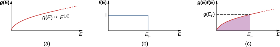$T=0\phantom{\rule{0.2em}{0ex}}\text{K}$ .

A few notes are in order. First, the electron number density (last row) distribution drops off sharply at the Fermi energy. According to the theory, this energy is given by

${E}_{\text{F}}=\frac{{h}^{2}}{8{m}_{e}}{\left(\frac{3N}{\pi V}\right)}^{2\text{/}3}.$

Fermi energies for selected materials are listed in the following table.

Conduction Electron Densities and Fermi Energies for Some Metals
Element	Conduction Band Electron Density $\left({10}^{28}\phantom{\rule{0.2em}{0ex}}{\text{m}}^{-3}\right)$	Free-Electron Model Fermi Energy $\left(\text{eV}\right)$
$\text{Al}$	$18.1$	$11.7$
$\text{Ba}$	$3.15$	$3.64$
$\text{Cu}$	$8.47$	$7.00$
$\text{Au}$	$5.90$	$5.53$
$\text{Fe}$	$17.0$	$11.1$
$\text{Ag}$	$5.86$	$5.49$

Note also that only the graph in part (c) of the figure, which answers the question, “How many particles are found in the energy range?” is checked by experiment. The Fermi temperature or effective “temperature” of an electron at the Fermi energy is

${T}_{\text{F}}=\frac{{E}_{\text{F}}}{{k}_{\text{B}}}.$

Fermi Energy of Silver Metallic silver is an excellent conductor. It has $5.86\phantom{\rule{0.2em}{0ex}}×\phantom{\rule{0.2em}{0ex}}{10}^{28}$ conduction electrons per cubic meter. (a) Calculate its Fermi energy. (b) Compare this energy to the thermal energy ${k}_{\text{B}}T$ of the electrons at a room temperature of 300 K.

Solution

From (Figure), the Fermi energy is

$\begin{array}{cc}{E}_{\text{F}}\hfill & =\frac{{h}^{2}}{2{m}_{e}}{\left(3{\pi }^{2}{n}_{e}\right)}^{2\text{/}3}\hfill \\ & =\frac{{\left(1.05\phantom{\rule{0.2em}{0ex}}×\phantom{\rule{0.2em}{0ex}}{10}^{-34}\phantom{\rule{0.2em}{0ex}}\text{J}·\text{s}\right)}^{2}}{2\left(9.11\phantom{\rule{0.2em}{0ex}}×\phantom{\rule{0.2em}{0ex}}{10}^{-31}\phantom{\rule{0.2em}{0ex}}\text{kg}\right)}\phantom{\rule{0.2em}{0ex}}×\phantom{\rule{0.2em}{0ex}}{\left[\left(3{\pi }^{2}\left(5.86\phantom{\rule{0.2em}{0ex}}×\phantom{\rule{0.2em}{0ex}}{10}^{28}\phantom{\rule{0.2em}{0ex}}{\text{m}}^{-3}\right)\right]}^{2\text{/}3}\hfill \\ & =8.79\phantom{\rule{0.2em}{0ex}}×\phantom{\rule{0.2em}{0ex}}{10}^{-19}\phantom{\rule{0.2em}{0ex}}\text{J}=5.49\phantom{\rule{0.2em}{0ex}}\text{eV}.\hfill \end{array}$

This is a typical value of the Fermi energy for metals, as can be seen from (Figure).
We can associate a Fermi temperature ${T}_{\text{F}}$ with the Fermi energy by writing ${k}_{\text{B}}{T}_{\text{F}}={E}_{\text{F}}.$ We then find for the Fermi temperature

${T}_{\text{F}}=\frac{8.79\phantom{\rule{0.2em}{0ex}}×\phantom{\rule{0.2em}{0ex}}{10}^{-19}\phantom{\rule{0.2em}{0ex}}\text{J}}{1.38\phantom{\rule{0.2em}{0ex}}×\phantom{\rule{0.2em}{0ex}}{10}^{-23}\phantom{\rule{0.2em}{0ex}}\text{J/K}}=6.37\phantom{\rule{0.2em}{0ex}}×\phantom{\rule{0.2em}{0ex}}{10}^{4}\phantom{\rule{0.2em}{0ex}}\text{K},$

which is much higher than room temperature and also the typical melting point $\left(\sim {10}^{3}\phantom{\rule{0.2em}{0ex}}\text{K}\right)$ of a metal. The ratio of the Fermi energy of silver to the room-temperature thermal energy is

$\frac{{E}_{\text{F}}}{{k}_{\text{B}}T}=\frac{{T}_{\text{F}}}{T}\approx 210.$

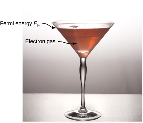
To visualize how the quantum states are filled, we might imagine pouring water slowly into a glass, such as that of (Figure). The first drops of water (the electrons) occupy the bottom of the glass (the states with lowest energy). As the level rises, states of higher and higher energy are occupied. Furthermore, since the glass has a wide opening and a narrow stem, more water occupies the top of the glass than the bottom. This reflects the fact that the density of states g(E) is proportional to ${E}^{1\text{/}2}$ , so there is a relatively large number of higher energy electrons in a free electron gas. Finally, the level to which the glass is filled corresponds to the Fermi energy.

An analogy of how electrons fill energy states in a metal. As electrons fill energy states, lowest to highest, the number of available states increases. The highest energy state (corresponding to the water line) is the Fermi energy. (credit: modification of work by “Didriks”/Flickr)

Photograph of a martini glass half filled with water. The water is labeled electron gas and the water line is labeled Fermi energy E subscript F.

Suppose that at $T=0\phantom{\rule{0.2em}{0ex}}\text{K}$ , the number of conduction electrons per unit volume in our sample is ${n}_{e}$ . Since each field state has one electron, the number of filled states per unit volume is the same as the number of electrons per unit volume.

Summary

Metals conduct electricity, and electricity is composed of large numbers of randomly colliding and approximately free electrons.
The allowed energy states of an electron are quantized. This quantization appears in the form of very large electron energies, even at $T=0\phantom{\rule{0.2em}{0ex}}\text{K}$ .
The allowed energies of free electrons in a metal depend on electron mass and on the electron number density of the metal.
The density of states of an electron in a metal increases with energy, because there are more ways for an electron to fill a high-energy state than a low-energy state.
Pauli’s exclusion principle states that only two electrons (spin up and spin down) can occupy the same energy level. Therefore, in filling these energy levels (lowest to highest at $T=0\phantom{\rule{0.2em}{0ex}}\text{K}\right),$ the last and largest energy level to be occupied is called the Fermi energy.

Conceptual Questions

Why does the Fermi energy $\left({E}_{\text{F}}\right)$ increase with the number of electrons in a metal?

If the electron number density (N/V) of a metal increases by a factor 8, what happens to the Fermi energy $\left({E}_{\text{F}}\right)?$

increases by a factor of $\sqrt[3]{{8}^{2}}=4$

Why does the horizontal line in the graph in (Figure) suddenly stop at the Fermi energy?

Why does the graph in (Figure) increase gradually from the origin?

For larger energies, the number of accessible states increases.

Why are the sharp transitions at the Fermi energy “smoothed out” by increasing the temperature?

Problems

What is the difference in energy between the ${n}_{x}={n}_{y}={n}_{z}=4$ state and the state with the next higher energy? What is the percentage change in the energy between the ${n}_{x}={n}_{y}={n}_{z}=4$ state and the state with the next higher energy? (b) Compare these with the difference in energy and the percentage change in the energy between the ${n}_{x}={n}_{y}={n}_{z}=400$ state and the state with the next higher energy.

a. $4%$ ; b. $4.2\phantom{\rule{0.2em}{0ex}}×\phantom{\rule{0.2em}{0ex}}{10}^{-4}%$ ; for very large values of the quantum numbers, the spacing between adjacent energy levels is very small (“in the continuum”). This is consistent with the expectation that for large quantum numbers, quantum and classical mechanics give approximately the same predictions.

An electron is confined to a metal cube of $l=0.8\phantom{\rule{0.2em}{0ex}}\text{cm}$ on each side. Determine the density of states at (a) $E=0.80\phantom{\rule{0.2em}{0ex}}\text{eV}$ ; (b) $E=2.2\phantom{\rule{0.2em}{0ex}}\text{eV}$ ; and (c) $E=5.0\phantom{\rule{0.2em}{0ex}}\text{eV}$ .

What value of energy corresponds to a density of states of $1.10\phantom{\rule{0.2em}{0ex}}×\phantom{\rule{0.2em}{0ex}}{10}^{24}\phantom{\rule{0.2em}{0ex}}{\text{eV}}^{-1}$ ?

10.0 eV

Compare the density of states at 2.5 eV and 0.25 eV.

Consider a cube of copper with edges 1.50 mm long. Estimate the number of electron quantum states in this cube whose energies are in the range 3.75 to 3.77 eV.

$4.55\phantom{\rule{0.2em}{0ex}}×\phantom{\rule{0.2em}{0ex}}{10}^{9}$

If there is one free electron per atom of copper, what is the electron number density of this metal?

Determine the Fermi energy and temperature for copper at $T=0\phantom{\rule{0.2em}{0ex}}\text{K}$ .

Fermi energy, ${E}_{\text{F}}=7.03\phantom{\rule{0.2em}{0ex}}\text{eV},$ Temperature, ${T}_{\text{F}}=8.2\phantom{\rule{0.2em}{0ex}}×\phantom{\rule{0.2em}{0ex}}{10}^{4}\phantom{\rule{0.2em}{0ex}}\text{K}$

Glossary

density of states: number of allowed quantum states per unit energy

electron number density: number of electrons per unit volume

Fermi energy: largest energy filled by electrons in a metal at $T=0\phantom{\rule{0.2em}{0ex}}\text{K}$

Fermi factor: number that expresses the probability that a state of given energy will be filled

Fermi temperature: effective temperature of electrons with energies equal to the Fermi energy

free electron model: model of a metal that views electrons as a gas

License

Icon for the Creative Commons Attribution 4.0 International License