
Quantum Mechanics
The Heisenberg Uncertainty Principle
Samuel J. Ling; Jeff Sanny; and William Moebs
Learning Objectives
By the end of this section, you will be able to:
- Describe the physical meaning of the position-momentum uncertainty relation
- Explain the origins of the uncertainty principle in quantum theory
- Describe the physical meaning of the energy-time uncertainty relation
Heisenberg’s uncertainty principle is a key principle in quantum mechanics. Very roughly, it states that if we know everything about where a particle is located (the uncertainty of position is small), we know nothing about its momentum (the uncertainty of momentum is large), and vice versa. Versions of the uncertainty principle also exist for other quantities as well, such as energy and time. We discuss the momentum-position and energy-time uncertainty principles separately.
Momentum and Position
To illustrate the momentum-position uncertainty principle, consider a free particle that moves along the x-direction. The particle moves with a constant velocity u and momentum  . According to de Broglie’s relations,
  and
and  . As discussed in the previous section, the wave function for this particle is given by
![{\psi }_{k}\left(x,t\right)=A\left[\text{cos}\left(\omega \text{ }t-k\text{ }x\right)-i\phantom{\rule{0.2em}{0ex}}\text{sin}\left(\omega \text{ }t-k\text{ }x\right)\right]=A{e}^{\text{−}i\left(\omega \text{ }t-k\text{ }x\right)}=A{e}^{\text{−}i\text{ }\omega \text{ }t}{e}^{i\text{ }k\text{ }x}](https://pressbooks.online.ucf.edu/app/uploads/quicklatex/quicklatex.com-c3833e1fde9c1cf109fb296d88e478f7_l3.png "Rendered by QuickLaTeX.com")
and the probability density  is uniform and independent of time. The particle is equally likely to be found anywhere along the x-axis but has definite values of wavelength and wave number, and therefore momentum. The uncertainty of position is infinite (we are completely uncertain about position) and the uncertainty of the momentum is zero (we are completely certain about momentum). This account of a free particle is consistent with Heisenberg’s uncertainty principle.
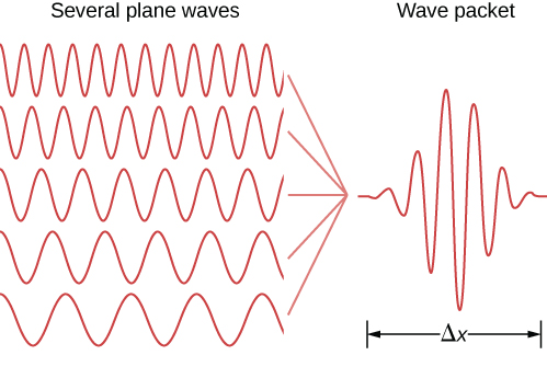
Similar statements can be made of localized particles. In quantum theory, a localized particle is modeled by a linear superposition of free-particle (or plane-wave) states called a wave packet. An example of a wave packet is shown in (Figure). A wave packet contains many wavelengths and therefore by de Broglie’s relations many momenta—possible in quantum mechanics! This particle also has many values of position, although the particle is confined mostly to the interval  . The particle can be better localized
  can be decreased) if more plane-wave states of different wavelengths or momenta are added together in the right way
  is increased). According to Heisenberg, these uncertainties obey the following relation.
The product of the uncertainty in position of a particle and the uncertainty in its momentum can never be less than one-half of the reduced Planck constant:

This relation expresses Heisenberg’s uncertainty principle. It places limits on what we can know about a particle from simultaneous measurements of position and momentum. If is large,  is small, and vice versa. (Figure) can be derived in a more advanced course in modern physics. Reflecting on this relation in his work The Physical Principles of the Quantum Theory, Heisenberg wrote “Any use of the words ‘position’ and ‘velocity’ with accuracy exceeding that given by [the relation] is just as meaningless as the use of words whose sense is not defined.”
Note that the uncertainty principle has nothing to do with the precision of an experimental apparatus. Even for perfect measuring devices, these uncertainties would remain because they originate in the wave-like nature of matter. The precise value of the product  depends on the specific form of the wave function. Interestingly, the Gaussian function (or bell-curve distribution) gives the minimum value of the uncertainty product:
The Uncertainty Principle Large and Small Determine the minimum uncertainties in the positions of the following objects if their speeds are known with a precision of  : (a) an electron and (b) a bowling ball of mass 6.0 kg.
Strategy Given the uncertainty in speed  , we have to first determine the uncertainty in momentum
  and then invert (Figure) to find the uncertainty in position
  .
.
Solution
- For the electron:

- For the bowling ball:

Significance Unlike the position uncertainty for the electron, the position uncertainty for the bowling ball is immeasurably small. Planck’s constant is very small, so the limitations imposed by the uncertainty principle are not noticeable in macroscopic systems such as a bowling ball.
Uncertainty and the Hydrogen Atom Estimate the ground-state energy of a hydrogen atom using Heisenberg’s uncertainty principle. (Hint: According to early experiments, the size of a hydrogen atom is approximately 0.1 nm.)
Strategy An electron bound to a hydrogen atom can be modeled by a particle bound to a one-dimensional box of length  The ground-state wave function of this system is a half wave, like that given in (Figure). This is the largest wavelength that can “fit” in the box, so the wave function corresponds to the lowest energy state. Note that this function is very similar in shape to a Gaussian (bell curve) function. We can take the average energy of a particle described by this function (E) as a good estimate of the ground state energy
  . This average energy of a particle is related to its average of the momentum squared, which is related to its momentum uncertainty.
Solution To solve this problem, we must be specific about what is meant by “uncertainty of position” and “uncertainty of momentum.” We identify the uncertainty of position  with the standard deviation of position
  , and the uncertainty of momentum
  with the standard deviation of momentum
  . For the Gaussian function, the uncertainty product is

where

The particle is equally likely to be moving left as moving right, so  . Also, the uncertainty of position is comparable to the size of the box, so
  The estimated ground state energy is therefore

Multiplying numerator and denominator by  gives
gives

Significance Based on early estimates of the size of a hydrogen atom and the uncertainty principle, the ground-state energy of a hydrogen atom is in the eV range. The ionization energy of an electron in the ground-state energy is approximately 10 eV, so this prediction is roughly confirmed. (Note: The product  is often a useful value in performing calculations in quantum mechanics.)
Energy and Time
Another kind of uncertainty principle concerns uncertainties in simultaneous measurements of the energy of a quantum state and its lifetime,

where  is the uncertainty in the energy measurement and
  is the uncertainty in the lifetime measurement. The energy-time uncertainty principle does not result from a relation of the type expressed by (Figure) for technical reasons beyond this discussion. Nevertheless, the general meaning of the energy-time principle is that a quantum state that exists for only a short time cannot have a definite energy. The reason is that the frequency of a state is inversely proportional to time and the frequency connects with the energy of the state, so to measure the energy with good precision, the state must be observed for many cycles.
To illustrate, consider the excited states of an atom. The finite lifetimes of these states can be deduced from the shapes of spectral lines observed in atomic emission spectra. Each time an excited state decays, the emitted energy is slightly different and, therefore, the emission line is characterized by a distribution of spectral frequencies (or wavelengths) of the emitted photons. As a result, all spectral lines are characterized by spectral widths. The average energy of the emitted photon corresponds to the theoretical energy of the excited state and gives the spectral location of the peak of the emission line. Short-lived states have broad spectral widths and long-lived states have narrow spectral widths.
Atomic Transitions An atom typically exists in an excited state for about  . Estimate the uncertainty
  in the frequency of emitted photons when an atom makes a transition from an excited state with the simultaneous emission of a photon with an average frequency of
  . Is the emitted radiation monochromatic?
Strategy We invert (Figure) to obtain the energy uncertainty  and combine it with the photon energy
  to obtain . To estimate whether or not the emission is monochromatic, we evaluate
  .
.
Solution The spread in photon energies is  . Therefore,

Significance Because the emitted photons have their frequencies within  percent of the average frequency, the emitted radiation can be considered monochromatic.
Check Your Understanding A sodium atom makes a transition from the first excited state to the ground state, emitting a 589.0-nm photon with energy 2.105 eV. If the lifetime of this excited state is  , what is the uncertainty in energy of this excited state? What is the width of the corresponding spectral line?
 ;
; 
Summary
- The Heisenberg uncertainty principle states that it is impossible to simultaneously measure the x-components of position and of momentum of a particle with an arbitrarily high precision. The product of experimental uncertainties is always larger than or equal to

- The limitations of this principle have nothing to do with the quality of the experimental apparatus but originate in the wave-like nature of matter.
- The energy-time uncertainty principle expresses the experimental observation that a quantum state that exists only for a short time cannot have a definite energy.
Conceptual Questions
If the formalism of quantum mechanics is ‘more exact’ than that of classical mechanics, why don’t we use quantum mechanics to describe the motion of a leaping frog? Explain.
Can the de Broglie wavelength of a particle be known precisely? Can the position of a particle be known precisely?
Yes, if its position is completely unknown. Yes, if its momentum is completely unknown.
Can we measure the energy of a free localized particle with complete precision?
Can we measure both the position and momentum of a particle with complete precision?
No. According to the uncertainty principle, if the uncertainty on the particle’s position is small, the uncertainty on its momentum is large. Similarly, if the uncertainty on the particle’s position is large, the uncertainty on its momentum is small.
Problems
A velocity measurement of an  -particle has been performed with a precision of 0.02 mm/s. What is the minimum uncertainty in its position?
A gas of helium atoms at 273 K is in a cubical container with 25.0 cm on a side. (a) What is the minimum uncertainty in momentum components of helium atoms? (b) What is the minimum uncertainty in velocity components? (c) Find the ratio of the uncertainties in (b) to the mean speed of an atom in each direction.
a.  ; b.
; b.  ; c.
; c. 
If the uncertainty in the  -component of a proton’s position is 2.0 pm, find the minimum uncertainty in the simultaneous measurement of the proton’s -component of velocity. What is the minimum uncertainty in the simultaneous measurement of the proton’s
  -component of velocity?
Some unstable elementary particle has a rest energy of 80.41 GeV and an uncertainty in rest energy of 2.06 GeV. Estimate the lifetime of this particle.

An atom in a metastable state has a lifetime of 5.2 ms. Find the minimum uncertainty in the measurement of energy of the excited state.
Measurements indicate that an atom remains in an excited state for an average time of 50.0 ns before making a transition to the ground state with the simultaneous emission of a 2.1-eV photon. (a) Estimate the uncertainty in the frequency of the photon. (b) What fraction of the photon’s average frequency is this?
a.  ; b.
; b. 
Suppose an electron is confined to a region of length 0.1 nm (of the order of the size of a hydrogen atom) and its kinetic energy is equal to the ground state energy of the hydrogen atom in Bohr’s model (13.6 eV). (a) What is the minimum uncertainty of its momentum? What fraction of its momentum is it? (b) What would the uncertainty in kinetic energy of this electron be if its momentum were equal to your answer in part (a)? What fraction of its kinetic energy is it?
Glossary
- Heisenberg’s uncertainty principle
- places limits on what can be known from a simultaneous measurements of position and momentum; states that if the uncertainty on position is small then the uncertainty on momentum is large, and vice versa
- wave packet
- superposition of many plane matter waves that can be used to represent a localized particle
- energy-time uncertainty principle
- energy-time relation for uncertainties in the simultaneous measurements of the energy of a quantum state and of its lifetime
