The Hydrogen Atom

Samuel J. Ling; Jeff Sanny; William Moebs

Atomic Structure

The Hydrogen Atom

Samuel J. Ling; Jeff Sanny; and William Moebs

Learning Objectives

By the end of this section, you will be able to:

Describe the hydrogen atom in terms of wave function, probability density, total energy, and orbital angular momentum
Identify the physical significance of each of the quantum numbers ( $n,l,m$ ) of the hydrogen atom
Distinguish between the Bohr and Schrödinger models of the atom
Use quantum numbers to calculate important information about the hydrogen atom

The hydrogen atom is the simplest atom in nature and, therefore, a good starting point to study atoms and atomic structure. The hydrogen atom consists of a single negatively charged electron that moves about a positively charged proton ((Figure)). In Bohr’s model, the electron is pulled around the proton in a perfectly circular orbit by an attractive Coulomb force. The proton is approximately 1800 times more massive than the electron, so the proton moves very little in response to the force on the proton by the electron. (This is analogous to the Earth-Sun system, where the Sun moves very little in response to the force exerted on it by Earth.) An explanation of this effect using Newton’s laws is given in Photons and Matter Waves.

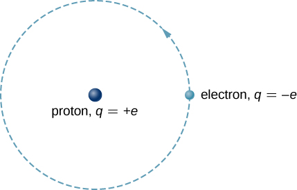
A representation of the Bohr model of the hydrogen atom.

The Bohr model of the hydrogen atom has the proton, charge q = plus e, at the center and the electron, charge q = minus e, in a circular orbit centered on the proton.

With the assumption of a fixed proton, we focus on the motion of the electron.

In the electric field of the proton, the potential energy of the electron is

$U\left(r\right)=\text{−}k\frac{{e}^{2}}{r},$

where $k=1\text{/}4\pi {\epsilon }_{0}$ and r is the distance between the electron and the proton. As we saw earlier, the force on an object is equal to the negative of the gradient (or slope) of the potential energy function. For the special case of a hydrogen atom, the force between the electron and proton is an attractive Coulomb force.

Notice that the potential energy function U(r) does not vary in time. As a result, Schrödinger’s equation of the hydrogen atom reduces to two simpler equations: one that depends only on space (x, y, z) and another that depends only on time (t). (The separation of a wave function into space- and time-dependent parts for time-independent potential energy functions is discussed in Quantum Mechanics.) We are most interested in the space-dependent equation:

$\frac{\text{−}{\hslash }^{2}}{2{m}_{e}}\left(\frac{{\partial }^{2}\psi }{\partial {x}^{2}}+\frac{{\partial }^{2}\psi }{\partial {y}^{2}}+\frac{{\partial }^{2}\psi }{\partial {z}^{2}}\right)-k\frac{{e}^{2}}{r}\psi =E\psi ,$

where $\psi =\psi \left(x,y,z\right)$ is the three-dimensional wave function of the electron, ${m}_{e}$ is the mass of the electron, and E is the total energy of the electron. Recall that the total wave function $\Psi \left(x,y,z,t\right),$ is the product of the space-dependent wave function $\psi =\psi \left(x,y,z\right)$ and the time-dependent wave function $\phi =\phi \left(t\right)$ .

In addition to being time-independent, U(r) is also spherically symmetrical. This suggests that we may solve Schrödinger’s equation more easily if we express it in terms of the spherical coordinates $\left(r\text{,}\phantom{\rule{0.2em}{0ex}}\theta \text{,}\phantom{\rule{0.2em}{0ex}}\varphi \right)$ instead of rectangular coordinates $\left(x,y,z\right)$ . A spherical coordinate system is shown in (Figure). In spherical coordinates, the variable r is the radial coordinate, $\theta$ is the polar angle (relative to the vertical z-axis), and $\varphi$ is the azimuthal angle (relative to the x-axis). The relationship between spherical and rectangular coordinates is $x=r\phantom{\rule{0.2em}{0ex}}\text{sin}\phantom{\rule{0.2em}{0ex}}\theta \phantom{\rule{0.2em}{0ex}}\text{cos}\phantom{\rule{0.2em}{0ex}}\varphi ,\phantom{\rule{0.5em}{0ex}}y=r\phantom{\rule{0.2em}{0ex}}\text{sin}\phantom{\rule{0.2em}{0ex}}\theta \phantom{\rule{0.2em}{0ex}}\text{sin}\phantom{\rule{0.2em}{0ex}}\varphi ,\phantom{\rule{0.5em}{0ex}}z=r\phantom{\rule{0.2em}{0ex}}\text{cos}\phantom{\rule{0.2em}{0ex}}\theta .$

The relationship between the spherical and rectangular coordinate systems.

An x y z coordinate system is shown, along with a point P and the vector r from the origin to P. In this figure, the point P has positive x, y, and z coordinates. The vector r is inclined by an angle theta from the positive z axis. Its projection on the x y plane makes an angle theta from the positive x axis toward the positive y axis.

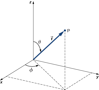
The factor $r\phantom{\rule{0.2em}{0ex}}\text{sin}\phantom{\rule{0.2em}{0ex}}\theta$ is the magnitude of a vector formed by the projection of the polar vector onto the xy-plane. Also, the coordinates of x and y are obtained by projecting this vector onto the x– and y-axes, respectively. The inverse transformation gives

$r=\sqrt{{x}^{2}+{y}^{2}+{z}^{2}},\phantom{\rule{0.5em}{0ex}}\theta ={\text{cos}}^{-1}\left(\frac{z}{r}\right),\phantom{\rule{0.5em}{0ex}}\varphi ={\text{cos}}^{-1}\left(\frac{x}{\sqrt{{x}^{2}+{y}^{2}}}\right).$

Schrödinger’s wave equation for the hydrogen atom in spherical coordinates is discussed in more advanced courses in modern physics, so we do not consider it in detail here. However, due to the spherical symmetry of U(r), this equation reduces to three simpler equations: one for each of the three coordinates $\left(r,\theta ,\phantom{\rule{0.2em}{0ex}}\text{and}\phantom{\rule{0.2em}{0ex}}\varphi \right).$ Solutions to the time-independent wave function are written as a product of three functions:

$\psi \left(r,\theta ,\varphi \right)=R\left(r\right)\text{Θ}\left(\text{θ}\right)\Phi \left(\varphi \right),$

where R is the radial function dependent on the radial coordinate r only; $\text{Θ}$ is the polar function dependent on the polar coordinate $\theta$ only; and $\text{Φ}$ is the phi function of $\varphi$ only. Valid solutions to Schrödinger’s equation $\psi \left(r,\theta ,\varphi \right)$ are labeled by the quantum numbers n, l, and m.

$\begin{array}{ccc}n:\hfill & & \text{principal quantum number}\hfill \\ l:\hfill & & \text{angular momentum quantum number}\hfill \\ m:\hfill & & \text{angular momentum projection quantum number}\hfill \end{array}$

(The reasons for these names will be explained in the next section.) The radial function R depends only on n and l; the polar function $\text{Θ}$ depends only on l and m; and the phi function $\text{Φ}$ depends only on m. The dependence of each function on quantum numbers is indicated with subscripts:

${\psi }_{nlm}\left(r,\theta ,\varphi \right)={R}_{nl}\left(r\right){\text{Θ}}_{lm}\left(\theta \right){\text{Φ}}_{m}\left(\varphi \right).$

Not all sets of quantum numbers (n, l, m) are possible. For example, the orbital angular quantum number l can never be greater or equal to the principal quantum number $n\left(l<n\right)$ . Specifically, we have

$\begin{array}{ccc}\hfill n& =\hfill & 1,2,3,\text{…}\hfill \\ \hfill l& =\hfill & 0,1,2,\text{…},\left(n-1\right)\hfill \\ \hfill m& =\hfill & \text{−}l,\left(\text{−}l+1\right),\text{…},0,\text{…},\left(+l-1\right),+l\hfill \end{array}$

Notice that for the ground state, $n=1$ , $l=0$ , and $m=0$ . In other words, there is only one quantum state with the wave function for $n=1$ , and it is ${\psi }_{100}$ . However, for $n=2$ , we have

$\begin{array}{c}l=0,\phantom{\rule{0.5em}{0ex}}m=0\hfill \\ l=1,\phantom{\rule{0.5em}{0ex}}m=-1,0,1.\hfill \end{array}$

Therefore, the allowed states for the $n=2$ state are ${\psi }_{200}$ , ${\psi }_{21-1},{\psi }_{210}$ , and ${\psi }_{211}$ . Example wave functions for the hydrogen atom are given in (Figure). Note that some of these expressions contain the letter i, which represents $\sqrt{-1}$ . When probabilities are calculated, these complex numbers do not appear in the final answer.

Wave Functions of the Hydrogen Atom
$n=1,l=0,{m}_{l}=0$	${\psi }_{100}=\frac{1}{\sqrt{\pi }}\phantom{\rule{0.3em}{0ex}}\frac{1}{{a}_{0}{}^{3\text{/}2}}{e}^{\text{−}r\text{/}{a}_{0}}$
$n=2,l=0,{m}_{l}=0$	${\psi }_{200}=\frac{1}{4\sqrt{2\pi }}\phantom{\rule{0.3em}{0ex}}\frac{1}{{a}_{0}{}^{3\text{/}2}}\left(2-\frac{r}{{a}_{0}}\right){e}^{\text{−}r\text{/}2{a}_{0}}$
$n=2,l=1,{m}_{l}=-1$	${\psi }_{21-1}=\frac{1}{8\sqrt{\pi }}\phantom{\rule{0.3em}{0ex}}\frac{1}{{a}_{0}{}^{3\text{/}2}}\phantom{\rule{0.3em}{0ex}}\frac{r}{{a}_{0}}{e}^{\text{−}r\text{/}2{a}_{0}}\text{sin}\phantom{\rule{0.2em}{0ex}}\theta {e}^{\text{−}i\varphi }$
$n=2,l=1,{m}_{l}=0$	${\psi }_{210}=\frac{1}{4\sqrt{2\pi }}\phantom{\rule{0.3em}{0ex}}\frac{1}{{a}_{0}{}^{3\text{/}2}}\phantom{\rule{0.3em}{0ex}}\frac{r}{{a}_{0}}{e}^{\text{−}r\text{/}2{a}_{0}}\text{cos}\phantom{\rule{0.2em}{0ex}}\theta$
$n=2,l=1,{m}_{l}=1$	${\psi }_{211}=\frac{1}{8\sqrt{\pi }}\phantom{\rule{0.3em}{0ex}}\frac{1}{{a}_{0}{}^{3\text{/}2}}\phantom{\rule{0.3em}{0ex}}\frac{r}{{a}_{0}}{e}^{\text{−}r\text{/}2{a}_{0}}\text{sin}\phantom{\rule{0.2em}{0ex}}\theta {e}^{i\varphi }$

Physical Significance of the Quantum Numbers

Each of the three quantum numbers of the hydrogen atom (n, l, m) is associated with a different physical quantity. The principal quantum number n is associated with the total energy of the electron, ${E}_{n}$ . According to Schrödinger’s equation:

${E}_{n}=\text{−}\left(\frac{{m}_{e}{k}^{2}{e}^{4}}{{2}^{2}}\right)\left(\frac{1}{{n}^{2}}\right)=\text{−}{E}_{0}\left(\frac{1}{{n}^{2}}\right),$

where ${E}_{0}=-13.6\phantom{\rule{0.2em}{0ex}}\text{eV}\text{.}$ Notice that this expression is identical to that of Bohr’s model. As in the Bohr model, the electron in a particular state of energy does not radiate.

How Many Possible States? For the hydrogen atom, how many possible quantum states correspond to the principal number $n=3$ ? What are the energies of these states?

Strategy For a hydrogen atom of a given energy, the number of allowed states depends on its orbital angular momentum. We can count these states for each value of the principal quantum number, $n=1,2,3.$ However, the total energy depends on the principal quantum number only, which means that we can use (Figure) and the number of states counted.

Solution If $n=3$ , the allowed values of l are 0, 1, and 2. If $l=0$ , $m=0$ (1 state). If $l=1$ , $m=-1,0,+1$ (3 states); and if $l=2$ , $m=-2,-1,0,+1,+2$ (5 states). In total, there are $1+3+5=9$ allowed states. Because the total energy depends only on the principal quantum number, $n=3$ , the energy of each of these states is

${E}_{n3}=\text{−}{E}_{0}\left(\frac{1}{{n}^{2}}\right)=\frac{-13.6\phantom{\rule{0.2em}{0ex}}\text{eV}}{9}=-1.51\phantom{\rule{0.2em}{0ex}}\text{eV}.$

Significance An electron in a hydrogen atom can occupy many different angular momentum states with the very same energy. As the orbital angular momentum increases, the number of the allowed states with the same energy increases.

The angular momentum orbital quantum number l is associated with the orbital angular momentum of the electron in a hydrogen atom. Quantum theory tells us that when the hydrogen atom is in the state ${\psi }_{nlm}$ , the magnitude of its orbital angular momentum is

$L=\sqrt{l\left(l+1\right)}\hslash ,$

where

$l=0,1,2,\text{…},\left(n-1\right).$

This result is slightly different from that found with Bohr’s theory, which quantizes angular momentum according to the rule $L=n,\text{where}\phantom{\rule{0.2em}{0ex}}n=1,2,3,\text{...}.$

Quantum states with different values of orbital angular momentum are distinguished using spectroscopic notation ((Figure)). The designations s, p, d, and f result from early historical attempts to classify atomic spectral lines. (The letters stand for sharp, principal, diffuse, and fundamental, respectively.) After f, the letters continue alphabetically.

The ground state of hydrogen is designated as the 1s state, where “1” indicates the energy level $\left(n=1\right)$ and “s” indicates the orbital angular momentum state ( $l=0$ ). When $n=2$ , l can be either 0 or 1. The $n=2$ , $l=0$ state is designated “2s.” The $n=2$ , $l=1$ state is designated “2p.” When $n=3$ , l can be 0, 1, or 2, and the states are 3s, 3p, and 3d, respectively. Notation for other quantum states is given in (Figure).

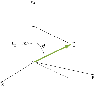
The angular momentum projection quantum number m is associated with the azimuthal angle $\varphi$ (see (Figure)) and is related to the z-component of orbital angular momentum of an electron in a hydrogen atom. This component is given by

${L}_{z}=m\hslash ,$

where

$m=\text{−}l,\text{−}l+1,\text{…},0,\text{…},+l-1,l.$

The z-component of angular momentum is related to the magnitude of angular momentum by

${L}_{z}=L\phantom{\rule{0.2em}{0ex}}cos\phantom{\rule{0.2em}{0ex}}\theta ,$

where $\theta$ is the angle between the angular momentum vector and the z-axis. Note that the direction of the z-axis is determined by experiment—that is, along any direction, the experimenter decides to measure the angular momentum. For example, the z-direction might correspond to the direction of an external magnetic field. The relationship between ${L}_{z}\text{and}\phantom{\rule{0.2em}{0ex}}L$ is given in (Figure).

The z-component of angular momentum is quantized with its own quantum number m.

An x y z coordinate system is shown. The vector L is at an angle theta to the positive z axis and has positive z component L sub z equal to m times h bar. The x and y components are positive but not specified.

Spectroscopic Notation and Orbital Angular Momentum
Orbital Quantum Number l	Angular Momentum	State	Spectroscopic Name
0	0	s	Sharp
1	$\sqrt{2}h$	p	Principal
2	$\sqrt{6}h$	d	Diffuse
3	$\sqrt{12}h$	f	Fundamental
4	$\sqrt{20}h$	g
5	$\sqrt{30}h$	h

Spectroscopic Description of Quantum States
	$l=0$	$l=1$	$l=2$	$l=3$	$l=4$	$l=5$
$n=1$	1s
$n=2$	2s	2p
$n=3$	3s	3p	3d
$n=4$	4s	4p	4d	4f
$n=5$	5s	5p	5d	5f	5g
$n=6$	6s	6p	6d	6f	6g	6h

The quantization of ${L}_{z}$ is equivalent to the quantization of $\theta$ . Substituting $\sqrt{l\left(l+1\right)}\hslash$ for L and m for ${L}_{z}$ into this equation, we find

$m\hslash =\sqrt{l\left(l+1\right)}\hslash \phantom{\rule{0.2em}{0ex}}\text{cos}\phantom{\rule{0.2em}{0ex}}\theta .$

Thus, the angle $\theta$ is quantized with the particular values

$\theta ={\text{cos}}^{-1}\left(\frac{m}{\sqrt{l\left(l+1\right)}}\right).$

Notice that both the polar angle ( $\theta$ ) and the projection of the angular momentum vector onto an arbitrary z-axis ( ${L}_{z}$ ) are quantized.

The quantization of the polar angle for the $l=3$ state is shown in (Figure). The orbital angular momentum vector lies somewhere on the surface of a cone with an opening angle $\theta$ relative to the z-axis (unless $m=0,$ in which case $\theta =90\text{°}$ and the vector points are perpendicular to the z-axis).

The quantization of orbital angular momentum. Each vector lies on the surface of a cone with axis along the z-axis.

A detailed study of angular momentum reveals that we cannot know all three components simultaneously. In the previous section, the z-component of orbital angular momentum has definite values that depend on the quantum number m. This implies that we cannot know both x- and y-components of angular momentum, ${L}_{x}$ and ${L}_{y}$ , with certainty. As a result, the precise direction of the orbital angular momentum vector is unknown.

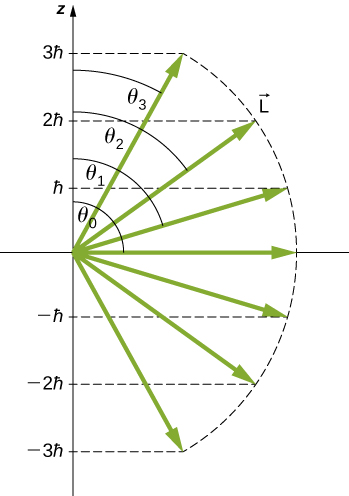
What Are the Allowed Directions? Calculate the angles that the angular momentum vector $\stackrel{\to }{L}$ can make with the z-axis for $l=1$ , as shown in (Figure).

The component of a given angular momentum along the z-axis (defined by the direction of a magnetic field) can have only certain values. These are shown here for $l=1$ , for which $m=-1,0,\text{and}+1.$ The direction of $\stackrel{\to }{L}$ is quantized in the sense that it can have only certain angles relative to the z-axis.

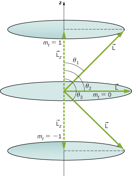
Strategy The vectors $\stackrel{\to }{L}$ and ${\stackrel{\to }{L}}_{z}$ (in the z-direction) form a right triangle, where $\stackrel{\to }{L}$ is the hypotenuse and ${\stackrel{\to }{L}}_{z}$ is the adjacent side. The ratio of ${L}_{z}$ to | $\stackrel{\to }{L}$ | is the cosine of the angle of interest. The magnitudes $L=|\stackrel{\to }{L}|$ and ${L}_{z}$ are given by

$L=\sqrt{l\left(l+1\right)}\hslash \phantom{\rule{0.2em}{0ex}}\text{and}\phantom{\rule{0.2em}{0ex}}{L}_{z}=m\hslash .$

Solution We are given $l=1$ , so ml can be $+1,0,\text{or}\phantom{\rule{0.2em}{0ex}}-1.$ Thus, L has the value given by

$L=\sqrt{l\left(l+1\right)}\hslash =\sqrt{2}\hslash .$

The quantity ${L}_{z}$ can have three values, given by ${L}_{z}={m}_{l}\hslash$ .

${L}_{z}={m}_{l}\hslash =\left\{\begin{array}{l}\phantom{\rule{0.5em}{0ex}}\hslash ,\text{}\phantom{\rule{0.2em}{0ex}}{m}_{l}=+1\hfill \\ \phantom{\rule{0.5em}{0ex}}0,\phantom{\rule{0.5em}{0ex}}{m}_{l}=0\hfill \\ -\hslash ,{m}_{l}=-1\hfill \end{array}$

As you can see in (Figure), $\text{cos}\phantom{\rule{0.2em}{0ex}}\theta ={L}_{z}\text{/}L,$ so for $m=+1$ , we have

$\text{cos}\phantom{\rule{0.2em}{0ex}}{\theta }_{1}=\frac{{L}_{Z}}{L}=\frac{\hslash }{\sqrt{2}\hslash }=\frac{1}{\sqrt{2}}=0.707.$

Thus,

${\theta }_{1}={\phantom{\rule{0.2em}{0ex}}\text{cos}}^{-1}0.707=45.0\text{°}.$

Similarly, for $m=0$ , we find $\text{cos}\phantom{\rule{0.2em}{0ex}}{\theta }_{2}=0;$ this gives

${\theta }_{2}={\text{cos}}^{-1}0=90.0\text{°}.$

Then for ${m}_{l}=-1$ :

$\text{cos}\phantom{\rule{0.2em}{0ex}}{\theta }_{3}=\frac{{L}_{Z}}{L}=\frac{\text{−}\hslash }{\sqrt{2}\hslash }=-\frac{1}{\sqrt{2}}=-0.707,$

so that

${\theta }_{3}={\phantom{\rule{0.2em}{0ex}}\text{cos}}^{-1}\left(-0.707\right)=135.0\text{°}.$

Significance The angles are consistent with the figure. Only the angle relative to the z-axis is quantized. L can point in any direction as long as it makes the proper angle with the z-axis. Thus, the angular momentum vectors lie on cones, as illustrated. To see how the correspondence principle holds here, consider that the smallest angle ( ${\theta }_{1}$ in the example) is for the maximum value of ${m}_{l},$ namely ${m}_{l}=l.$ For that smallest angle,

$\text{cos}\phantom{\rule{0.2em}{0ex}}\theta =\frac{{L}_{z}}{L}=\frac{l}{\sqrt{l\left(l+1\right)}},$

which approaches 1 as l becomes very large. If $\text{cos}\phantom{\rule{0.2em}{0ex}}\theta =1$ , then $\theta =0º$ . Furthermore, for large l, there are many values of ${m}_{l}$ , so that all angles become possible as l gets very large.

Check Your Understanding Can the magnitude of ${L}_{z}$ ever be equal to L?

No. The quantum number $m=\text{−}l,\text{−}l+1\text{,…},0\text{,…},l-1,l.$ Thus, the magnitude of ${L}_{z}$ is always less than L because $<\sqrt{l\left(l+1\right)}$

Using the Wave Function to Make Predictions

As we saw earlier, we can use quantum mechanics to make predictions about physical events by the use of probability statements. It is therefore proper to state, “An electron is located within this volume with this probability at this time,” but not, “An electron is located at the position (x, y, z) at this time.” To determine the probability of finding an electron in a hydrogen atom in a particular region of space, it is necessary to integrate the probability density $|{\psi }_{nlm}{|}^{2}$ over that region:

$\text{Probability}={\int }_{\text{volume}}|{\psi }_{nlm}{|}^{2}dV,$

where dV is an infinitesimal volume element. If this integral is computed for all space, the result is 1, because the probability of the particle to be located somewhere is 100% (the normalization condition). In a more advanced course on modern physics, you will find that $|{\psi }_{nlm}{|}^{2}={\psi }_{nlm}^{*}{\psi }_{nlm},$ where ${\psi }_{nlm}^{*}$ is the complex conjugate. This eliminates the occurrences of $i=\sqrt{-1}$ in the above calculation.

Consider an electron in a state of zero angular momentum ( $l=0$ ). In this case, the electron’s wave function depends only on the radial coordinate r. (Refer to the states ${\psi }_{100}$ and ${\psi }_{200}$ in (Figure).) The infinitesimal volume element corresponds to a spherical shell of radius r and infinitesimal thickness dr, written as

$dV=4\pi {r}^{2}dr.$

The probability of finding the electron in the region r to $r+dr$ (“at approximately r”) is

$P\left(r\right)dr=|{\psi }_{n00}{|}^{2}4\pi {r}^{2}dr.$

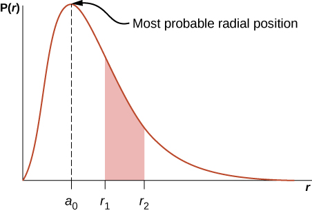
Here P(r) is called the radial probability density function (a probability per unit length). For an electron in the ground state of hydrogen, the probability of finding an electron in the region r to $r+dr$ is

$|{\psi }_{n00}{|}^{2}4\pi {r}^{2}dr=\left(4\text{/}{a}_{0}^{3}\right){r}^{2}\phantom{\rule{0.2em}{0ex}}\text{exp}\left(-2r\text{/}{a}_{0}\right)dr,$

where ${a}_{0}=0.5$ angstroms. The radial probability density function P(r) is plotted in (Figure). The area under the curve between any two radial positions, say ${r}_{1}$ and ${r}_{2}$ , gives the probability of finding the electron in that radial range. To find the most probable radial position, we set the first derivative of this function to zero ( $dP\text{/}dr=0$ ) and solve for r. The most probable radial position is not equal to the average or expectation value of the radial position because $|{\psi }_{n00}{|}^{2}$ is not symmetrical about its peak value.

The radial probability density function for the ground state of hydrogen.

A graph of the function P of r as a function of r is shown. It is zero at r = 0, rises to a maximum at r = a sub 0, then gradually decreases and goes asymptotically to zero at large r. The maximum is at the most probable radial position. The area of the region under the curve from r sub 1 to r sub 2 is shaded.

If the electron has orbital angular momentum ( $l\ne 0$ ), then the wave functions representing the electron depend on the angles $\theta$ and $\varphi ;$ that is, ${\psi }_{nlm}=$ ${\psi }_{nlm}$ (r, $\theta$ , $\varphi$ ). Atomic orbitals for three states with $n=2$ and $l=1$ are shown in (Figure). An atomic orbital is a region in space that encloses a certain percentage (usually 90%) of the electron probability. (Sometimes atomic orbitals are referred to as “clouds” of probability.) Notice that these distributions are pronounced in certain directions. This directionality is important to chemists when they analyze how atoms are bound together to form molecules.

The probability density distributions for three states with $n=2$ and $l=1$ . The distributions are directed along the (a) x-axis, (b) y-axis, and (c) z-axis.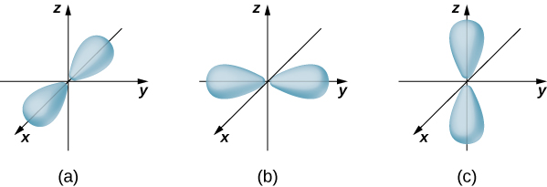

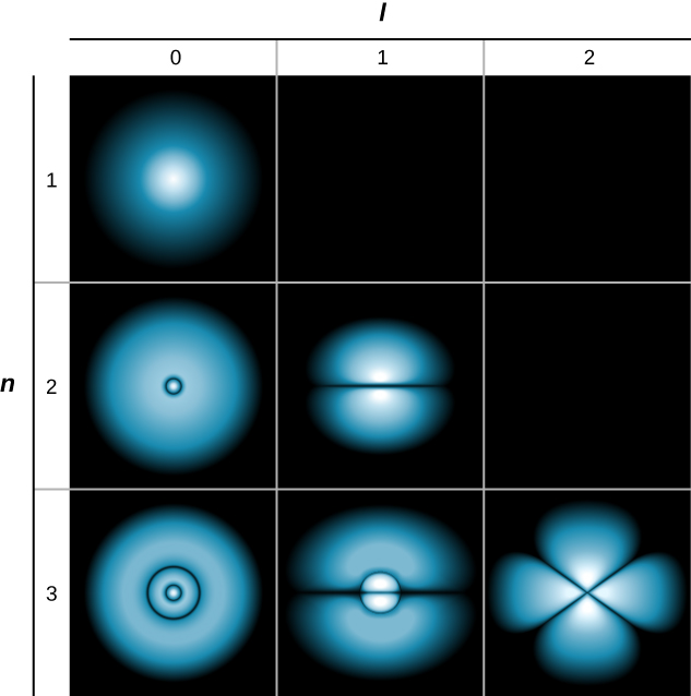
This diagram illustrates the shapes of p orbitals. The orbitals are dumbbell shaped and oriented along the x, y, and z axes.

A slightly different representation of the wave function is given in (Figure). In this case, light and dark regions indicate locations of relatively high and low probability, respectively. In contrast to the Bohr model of the hydrogen atom, the electron does not move around the proton nucleus in a well-defined path. Indeed, the uncertainty principle makes it impossible to know how the electron gets from one place to another.

Probability clouds for the electron in the ground state and several excited states of hydrogen. The probability of finding the electron is indicated by the shade of color; the lighter the coloring, the greater the chance of finding the electron.

Summary

A hydrogen atom can be described in terms of its wave function, probability density, total energy, and orbital angular momentum.
The state of an electron in a hydrogen atom is specified by its quantum numbers (n, l, m).
In contrast to the Bohr model of the atom, the Schrödinger model makes predictions based on probability statements.
The quantum numbers of a hydrogen atom can be used to calculate important information about the atom.

Conceptual Questions

Identify the physical significance of each of the quantum numbers of the hydrogen atom.

n (principal quantum number) $\to$ total energy
$l$ (orbital angular quantum number) $\to$ total absolute magnitude of the orbital angular momentum
m (orbital angular projection quantum number) $\to$ z-component of the orbital angular momentum

Describe the ground state of hydrogen in terms of wave function, probability density, and atomic orbitals.

Distinguish between Bohr’s and Schrödinger’s model of the hydrogen atom. In particular, compare the energy and orbital angular momentum of the ground states.

The Bohr model describes the electron as a particle that moves around the proton in well-defined orbits. Schrödinger’s model describes the electron as a wave, and knowledge about the position of the electron is restricted to probability statements. The total energy of the electron in the ground state (and all excited states) is the same for both models. However, the orbital angular momentum of the ground state is different for these models. In Bohr’s model, $L\left(\text{ground state}\right)=1$ , and in Schrödinger’s model, $L\left(\text{ground state}\right)=0$ .

Problems

The wave function is evaluated at rectangular coordinates ( $x,y,z$ ) $=$ (2, 1, 1) in arbitrary units. What are the spherical coordinates of this position?

$\left(r,\theta ,\varphi \right)=\left(\sqrt{6,}66\text{°},27\text{°}\right).$

If an atom has an electron in the $n=5$ state with $m=3$ , what are the possible values of l?

What are the possible values of m for an electron in the $n=4$ state?

$±3,±2,±1,0$ are possible

What, if any, constraints does a value of $m=1$ place on the other quantum numbers for an electron in an atom?

What are the possible values of m for an electron in the $n=4$ state?

$±3,±2,±1,0$ are possible

(a) How many angles can L make with the z-axis for an $l=2$ electron? (b) Calculate the value of the smallest angle.

The force on an electron is “negative the gradient of the potential energy function.” Use this knowledge and (Figure) to show that the force on the electron in a hydrogen atom is given by Coulomb’s force law.

$F=\text{−}k\frac{Qq}{{r}^{2}}$

What is the total number of states with orbital angular momentum $l=0$ ? (Ignore electron spin.)

The wave function is evaluated at spherical coordinates $\left(r,\theta ,\varphi \right)=\left(\sqrt{3},45\text{°},45\text{°}\right),$ where the value of the radial coordinate is given in arbitrary units. What are the rectangular coordinates of this position?

(1, 1, 1)

Coulomb’s force law states that the force between two charged particles is:

$F=k\frac{Qq}{{r}^{2}}.$ Use this expression to determine the potential energy function.

Write an expression for the total number of states with orbital angular momentum l.

For the orbital angular momentum quantum number, l, the allowed values of:
$m=\text{−}l,\text{−}l+1\text{,...}\phantom{\rule{0.2em}{0ex}}0\text{,...}\phantom{\rule{0.2em}{0ex}}l-1,l$ .
With the exception of $m=0$ , the total number is just 2l because the number of states on either side of $m=0$ is just l. Including $m=0$ , the total number of orbital angular momentum states for the orbital angular momentum quantum number, l, is: $2l+1.$ Later, when we consider electron spin, the total number of angular momentum states will be found to twice this value because each orbital angular momentum states is associated with two states of electron spin: spin up and spin down).

Consider hydrogen in the ground state, ${\psi }_{100}$ . (a) Use the derivative to determine the radial position for which the probability density, P(r), is a maximum.

(b) Use the integral concept to determine the average radial position. (This is called the expectation value of the electron’s radial position.) Express your answers into terms of the Bohr radius, ${a}_{o}$ . Hint: The expectation value is the just average value. (c) Why are these values different?

What is the probability that the 1s electron of a hydrogen atom is found outside the Bohr radius?

The probability that the 1s electron of a hydrogen atom is found outside of the Bohr radius is ${\int }_{{a}_{0}}^{\infty }P\left(r\right)dr\approx 0.68$

How many polar angles are possible for an electron in the $l=5$ state?

What is the maximum number of orbital angular momentum electron states in the $n=2$ shell of a hydrogen atom? (Ignore electron spin.)

For $n=2$ , $l=0$ (1 state), and $l=1$ (3 states). The total is 4.

What is the maximum number of orbital angular momentum electron states in the $n=3$ shell of a hydrogen atom? (Ignore electron spin.)

Glossary

angular momentum orbital quantum number (l): quantum number associated with the orbital angular momentum of an electron in a hydrogen atom

angular momentum projection quantum number (m): quantum number associated with the z-component of the orbital angular momentum of an electron in a hydrogen atom

atomic orbital: region in space that encloses a certain percentage (usually 90%) of the electron probability

principal quantum number (n): quantum number associated with the total energy of an electron in a hydrogen atom

radial probability density function: function use to determine the probability of a electron to be found in a spatial interval in r

License

Icon for the Creative Commons Attribution 4.0 International License