
Chapter 1 The Nature of Science and Physics
1.3 Accuracy, Precision, and Significant Figures
Summary
- Determine the appropriate number of significant figures in both addition and subtraction, as well as multiplication and division calculations.
- Calculate the percent uncertainty of a measurement.
Accuracy and Precision of a Measurement
Science is based on observation and experiment—that is, on measurements. Accuracy is how close a measurement is to the correct value for that measurement. For example, let us say that you are measuring the length of standard computer paper. The packaging in which you purchased the paper states that it is 11.0 inches long. You measure the length of the paper three times and obtain the following measurements: 11.1 in., 11.2 in., and 10.9 in. These measurements are quite accurate because they are very close to the correct value of 11.0 inches. In contrast, if you had obtained a measurement of 12 inches, your measurement would not be very accurate.
The precision of a measurement system is refers to how close the agreement is between repeated measurements (which are repeated under the same conditions). Consider the example of the paper measurements. The precision of the measurements refers to the spread of the measured values. One way to analyze the precision of the measurements would be to determine the range, or difference, between the lowest and the highest measured values. In that case, the lowest value was 10.9 in. and the highest value was 11.2 in. Thus, the measured values deviated from each other by at most 0.3 in. These measurements were relatively precise because they did not vary too much in value. However, if the measured values had been 10.9, 11.1, and 11.9, then the measurements would not be very precise because there would be significant variation from one measurement to another.
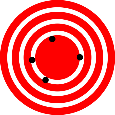
The measurements in the paper example are both accurate and precise, but in some cases, measurements are accurate but not precise, or they are precise but not accurate. Let us consider an example of a GPS system that is attempting to locate the position of a restaurant in a city. Think of the restaurant location as existing at the center of a bull’s-eye target, and think of each GPS attempt to locate the restaurant as a black dot. In Figure 3, you can see that the GPS measurements are spread out far apart from each other, but they are all relatively close to the actual location of the restaurant at the center of the target. This indicates a low precision, high accuracy measuring system. However, in Figure 4, the GPS measurements are concentrated quite closely to one another, but they are far away from the target location. This indicates a high precision, low accuracy measuring system.

Accuracy, Precision, and Uncertainty
The degree of accuracy and precision of a measuring system are related to the uncertainty in the measurements. Uncertainty is a quantitative measure of how much your measured values deviate from a standard or expected value. If your measurements are not very accurate or precise, then the uncertainty of your values will be very high. In more general terms, uncertainty can be thought of as a disclaimer for your measured values. For example, if someone asked you to provide the mileage on your car, you might say that it is 45,000 miles, plus or minus 500 miles. The plus or minus amount is the uncertainty in your value. That is, you are indicating that the actual mileage of your car might be as low as 44,500 miles or as high as 45,500 miles, or anywhere in between. All measurements contain some amount of uncertainty. In our example of measuring the length of the paper, we might say that the length of the paper is 11 in., plus or minus 0.2 in. The uncertainty in a measurement, [latex]{A}[/latex], is often denoted as [latex]{\delta}{A}[/latex] (“delta [latex]{A}[/latex] ”), so the measurement result would be recorded as [latex]{A}{\pm\delta}{A}[/latex]. In our paper example, the length of the paper could be expressed as [latex]{11\text{ in.}\pm 0.2}[/latex].
The factors contributing to uncertainty in a measurement include:
- Limitations of the measuring device,
- The skill of the person making the measurement,
- Irregularities in the object being measured,
- Any other factors that affect the outcome (highly dependent on the situation).
In our example, such factors contributing to the uncertainty could be the following: the smallest division on the ruler is 0.1 in., the person using the ruler has bad eyesight, or one side of the paper is slightly longer than the other. At any rate, the uncertainty in a measurement must be based on a careful consideration of all the factors that might contribute and their possible effects.
MAKING CONNECTIONS: REAL-WORLD CONNECTIONS – FEVER OR CHILLS?
Uncertainty is a critical piece of information, both in physics and in many other real-world applications. Imagine you are caring for a sick child. You suspect the child has a fever, so you check his or her temperature with a thermometer. What if the uncertainty of the thermometer were [latex]{3.0^{\text{o}}\text{C}}[/latex] ? If the child’s temperature reading was [latex]{37.0^{\text{o}}\text{C}}[/latex] (which is normal body temperature), the “true” temperature could be anywhere from a hypothermic [latex]{34.0^{\text{o}}\text{C}}[/latex] to a dangerously high [latex]{40.0^{\text{o}}\text{C}}[/latex]. A thermometer with an uncertainty of [latex]{3.0^{\text{o}}\text{C}}[/latex] would be useless.
Percent Uncertainty
One method of expressing uncertainty is as a percent of the measured value. If a measurement [latex]{A}[/latex] is expressed with uncertainty, [latex]{\delta{A,}}[/latex] the percent uncertainty (%unc) is defined to be:
Example 1: Calculating Percent Uncertainty: A Bag of Apples
A grocery store sells [latex]{5\text{-lb}}[/latex] bags of apples. You purchase four bags over the course of a month and weigh the apples each time. You obtain the following measurements:
- Week 1 weight: [latex]{4.8\text{ lb}}[/latex]
- Week 2 weight: [latex]{5.3\text{ lb}}[/latex]
- Week 3 weight: [latex]{4.9\text{ lb}}[/latex]
- Week 4 weight: [latex]{5.4\text{ lb}}[/latex]
You determine that the weight of the [latex]{5\text{-lb}}[/latex] bag has an uncertainty of [latex]{\pm0.4\text{ lb.}}[/latex] What is the percent uncertainty of the bag’s weight?
Strategy
First, observe that the expected value of the bag’s weight, [latex]{A}[/latex], is 5 lb. The uncertainty in this value, [latex]{\delta}{A}[/latex], is 0.4 lb. We can use the following equation to determine the percent uncertainty of the weight:
Solution
Plug the known values into the equation:
Discussion
We can conclude that the weight of the apple bag is [latex]{5\text{ lb}\pm8\%}[/latex]. Consider how this percent uncertainty would change if the bag of apples were half as heavy, but the uncertainty in the weight remained the same. Hint for future calculations: when calculating percent uncertainty, always remember that you must multiply the fraction by 100%. If you do not do this, you will have a decimal quantity, not a percent value.
Uncertainties in Calculations
There is an uncertainty in anything calculated from measured quantities. For example, the area of a floor calculated from measurements of its length and width has an uncertainty because the length and width have uncertainties. How big is the uncertainty in something you calculate by multiplication or division? If the measurements going into the calculation have small uncertainties (a few percent or less), then the method of adding percents can be used for multiplication or division. This method says that the percent uncertainty in a quantity calculated by multiplication or division is the sum of the percent uncertainties in the items used to make the calculation. For example, if a floor has a length of [latex]{4.00\text{ m}}[/latex] and a width of [latex]{3.00}\text{ m,}[/latex] with uncertainties of [latex]{2}{\%}[/latex] and [latex]{1}{\%}[/latex], respectively, then the area of the floor is [latex]{12.0\text{ m}^2}[/latex] and has an uncertainty of [latex]{3}{\%}[/latex]. (Expressed as an area this is [latex]{0.36\text{ m}^2}[/latex], which we round to [latex]{0.4\text{ m}^2}[/latex] since the area of the floor is given to a tenth of a square meter.)
Check Your Understanding 1
Precision of Measuring Tools and Significant Figures
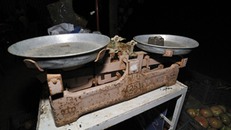
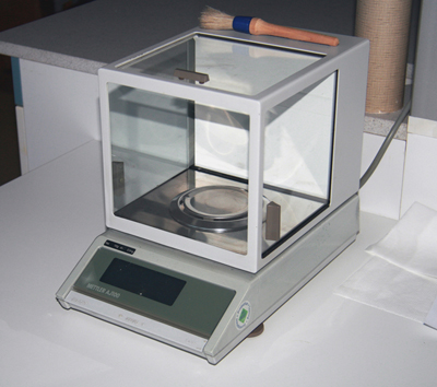
An important factor in the accuracy and precision of measurements involves the precision of the measuring tool. In general, a precise measuring tool is one that can measure values in very small increments. For example, a standard ruler can measure length to the nearest millimeter, while a caliper can measure length to the nearest 0.01 millimeter. The caliper is a more precise measuring tool because it can measure extremely small differences in length. The more precise the measuring tool, the more precise and accurate the measurements can be.
When we express measured values, we can only list as many digits as we initially measured with our measuring tool. For example, if you use a standard ruler to measure the length of a stick, you may measure it to be [latex]{36.7}\text{ cm}[/latex]. You could not express this value as [latex]{36.71}\text{ cm}[/latex] because your measuring tool was not precise enough to measure a hundredth of a centimeter. It should be noted that the last digit in a measured value has been estimated in some way by the person performing the measurement. For example, the person measuring the length of a stick with a ruler notices that the stick length seems to be somewhere in between [latex]{36.6}\text{ cm}[/latex] and [latex]{36.7}\text{ cm}[/latex], and he or she must estimate the value of the last digit. Using the method of significant figures, the rule is that the last digit written down in a measurement is the first digit with some uncertainty. In order to determine the number of significant digits in a value, start with the first measured value at the left and count the number of digits through the last digit written on the right. For example, the measured value [latex]{36.7}\text{ cm}[/latex] has three digits, or significant figures. Significant figures indicate the precision of a measuring tool that was used to measure a value.
Zeros
Special consideration is given to zeros when counting significant figures. The zeros in 0.053 are not significant, because they are only placekeepers that locate the decimal point. There are two significant figures in 0.053. The zeros in 10.053 are not placekeepers but are significant—this number has five significant figures. The zeros in 1300 may or may not be significant depending on the style of writing numbers. They could mean the number is known to the last digit, or they could be placekeepers. So 1300 could have two, three, or four significant figures. (To avoid this ambiguity, write 1300 in scientific notation.) Zeros are significant except when they serve only as placekeepers.
Check Your Understanding 2
Significant Figures in Calculations
When combining measurements with different degrees of accuracy and precision, the number of significant digits in the final answer can be no greater than the number of significant digits in the least precise measured value. There are two different rules, one for multiplication and division and the other for addition and subtraction, as discussed below.
1. For multiplication and division: The result should have the same number of significant figures as the quantity having the least significant figures entering into the calculation. For example, the area of a circle can be calculated from its radius using [latex]{A}{=\pi{r}^2}[/latex]. Let us see how many significant figures the area has if the radius has only two—say, [latex]{r=1.2}\text{ m.}[/latex] Then,
is what you would get using a calculator that has an eight-digit output. But because the radius has only two significant figures, it limits the calculated quantity to two significant figures or
even though [latex]{\pi}[/latex] is good to at least eight digits.
2. For addition and subtraction: The answer can contain no more decimal places than the least precise measurement. Suppose that you buy 7.56-kg of potatoes in a grocery store as measured with a scale with precision 0.01 kg. Then you drop off 6.052-kg of potatoes at your laboratory as measured by a scale with precision 0.001 kg. Finally, you go home and add 13.7 kg of potatoes as measured by a bathroom scale with precision 0.1 kg. How many kilograms of potatoes do you now have, and how many significant figures are appropriate in the answer? The mass is found by simple addition and subtraction:
Next, we identify the least precise measurement: 13.7 kg. This measurement is expressed to the 0.1 decimal place, so our final answer must also be expressed to the 0.1 decimal place. Thus, the answer is rounded to the tenths place, giving us 15.2 kg.
Significant Figures in this Text
In this text, most numbers are assumed to have three significant figures. Furthermore, consistent numbers of significant figures are used in all worked examples. You will note that an answer given to three digits is based on input good to at least three digits, for example. If the input has fewer significant figures, the answer will also have fewer significant figures. Care is also taken that the number of significant figures is reasonable for the situation posed. In some topics, particularly in optics, more accurate numbers are needed and more than three significant figures will be used. Finally, if a number is exact, such as the two in the formula for the circumference of a circle, [latex]{c}{=2\pi{r}}[/latex], it does not affect the number of significant figures in a calculation.
Check Your Understanding 3
PHET EXPLORATION: ESTIMATION
Explore size estimation in one, two, and three dimensions! Multiple levels of difficulty allow for progressive skill improvement.
Summary
- Accuracy of a measured value refers to how close a measurement is to the correct value. The uncertainty in a measurement is an estimate of the amount by which the measurement result may differ from this value.
- Precision of measured values refers to how close the agreement is between repeated measurements.
- The precision of a measuring tool is related to the size of its measurement increments. The smaller the measurement increment, the more precise the tool.
- Significant figures express the precision of a measuring tool.
- When multiplying or dividing measured values, the final answer can contain only as many significant figures as the least precise value.
- When adding or subtracting measured values, the final answer cannot contain more decimal places than the least precise value.
Conceptual Questions
1: What is the relationship between the accuracy and uncertainty of a measurement?
2: Prescriptions for vision correction are given in units called diopters (D). Determine the meaning of that unit. Obtain information (perhaps by calling an optometrist or performing an internet search) on the minimum uncertainty with which corrections in diopters are determined and the accuracy with which corrective lenses can be produced. Discuss the sources of uncertainties in both the prescription and accuracy in the manufacture of lenses.
Problems & Exercises
Express your answer to problems in this section to the correct number of significant figures and proper units.
1: Suppose that your bathroom scale reads your mass as 65 kg with a 3% uncertainty. What is the uncertainty in your mass (in kilograms)?
3: (a) A car speedometer has a [latex]{5.0\%}[/latex] uncertainty. What is the range of possible speeds when it reads [latex]{90\text{ km/h}}[/latex] ? (b) Convert this range to miles per hour. [latex]{(1\text{ km} = 0.6214\text{ mi})}[/latex]
5: (a) Suppose that a person has an average heart rate of 72.0 beats/min. How many beats does he or she have in 2.0 y? (b) In 2.00 y? (c) In 2.000 y?
7: State how many significant figures are proper in the results of the following calculations: (a) [latex]{(106.7)(98.2)\backslash(46.210)(1.01)}[/latex] (b) [latex]{(18.7)^2}[/latex] (c) [latex]{(1.60\times 10^{-19}) (3712)}[/latex].
9: (a) If your speedometer has an uncertainty of [latex]{2.0\text{ km/h}}[/latex] at a speed of [latex]{90\text{ km/h}}[/latex], what is the percent uncertainty? (b) If it has the same percent uncertainty when it reads [latex]{60\text{ km/h}}[/latex], what is the range of speeds you could be going?
11: A person measures his or her heart rate by counting the number of beats in [latex]{30}\text{ s}[/latex]. If [latex]{40 \pm 1}[/latex] beats are counted in [latex]{30.0 \pm 0.5\text{ s}}[/latex], what is the heart rate and its uncertainty in beats per minute?
13: If a marathon runner averages 9.5 mi/h, how long does it take him or her to run a 26.22-mi marathon?
15: The sides of a small rectangular box are measured to be [latex]{1.80 \pm 0.01\text{ cm}}[/latex], [latex]{2.05 \pm 0.0\text{ 2cm}}[/latex], and [latex]{3.1 \pm 0.1\text{ cm}}[/latex] long. Calculate its volume and uncertainty in cubic centimeters.
17: The length and width of a rectangular room are measured to be [latex]{3.955 \pm 0.005\text{ m}}[/latex] and [latex]{3.050 \pm 0.005\text{ m}}[/latex]. Calculate the area of the room and its uncertainty in square meters.
Glossary
- accuracy
- the degree to which a measure value agrees with the correct value for that measurement
- method of adding percents
- the percent uncertainty in a quantity calculated by multiplication or division is the sum of the percent uncertainties in the items used to make the calculation
- percent uncertainty
- the ratio of the uncertainty of a measurement to the measure value, express as a percentage
- precision
- the degree to which repeated measurements agree with each other
- significant figures
- express the precision of a measuring tool used to measure a value
- uncertainty
- a quantitative measure of how much your measured values deviate from a standard or expected value
Solutions
Problems & Exercises
1: 2 kg
3: (a) [latex]{85.5\text{ to }94.5\text{ km/h}}[/latex], (b) [latex]{53.1\text{ to }58.7\text{ mi/h}}[/latex]
5: (a) [latex]{7.6\times10^6\text{ beats}}[/latex], (b) [latex]{7.57\times10^7\text{ beats}}[/latex], (c) [latex]{7.57\times10^7\text{ beats}}[/latex]
7: (a) 3, (b) 3, (c) 3
9: (a) [latex]{2.2\%}[/latex], (b) [latex]{59\text{ to }61\text{ km/h}}[/latex]
11: [latex]{80\pm3\text{ beats/min}}[/latex]
13: [latex]{2.8\text{ h}}[/latex]
15: [latex]{11.1 \pm 1\text{ m}^3}[/latex]
17: [latex]{12.06\pm0.04\text{ m}^2}[/latex]
the degree to which a measure value agrees with the correct value for that measurement
the degree to which repeated measurements agree with each other
a quantitative measure of how much your measured values deviate from a standard or expected value
the ratio of the uncertainty of a measurement to the measure value, express as a percentage
the percent uncertainty in a quantity calculated by multiplication or division is the sum of the percent uncertainties in the items used to make the calculation
express the precision of a measuring tool used to measure a value
