
45.1 and 45.2 Population Ecology and Life Histories
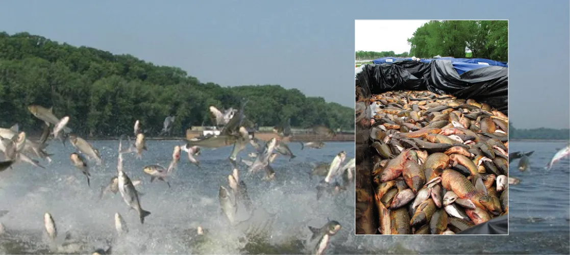
Imagine sailing down a river in a small motorboat on a weekend afternoon; the water is smooth and you are enjoying the warm sunshine and cool breeze when suddenly you are hit in the head by a 20-pound silver carp. This is now a risk on many rivers and canal systems in Illinois and Missouri because of the presence of Asian carp.
This fish—actually a group of species including the silver, black, grass, and big head carp—has been farmed and eaten in China for over 1000 years. It is one of the most important aquaculture food resources worldwide. In the United States, however, Asian carp is considered a dangerous invasive species that disrupts community structure and composition to the point of threatening native species.
Learning Objectives
- Describe how ecologists measure population size and density
- Describe three different patterns of population distribution
- Describe the three types of survivorship curves and relate them to specific populations
Populations are dynamic entities. A Population is a group of the same species living within a specific area, and populations fluctuate based on a number of factors: seasonal and yearly changes in the environment, natural disasters such as forest fires and volcanic eruptions, and competition for resources between and within species. The statistical study of population dynamics, demography, uses a series of mathematical tools to investigate how populations respond to changes in their biotic and abiotic environments. Many of these tools were originally designed to study human populations. For example, life tables, which detail the life expectancy of individuals within a population, were initially developed by life insurance companies to set insurance rates. In fact, while the term “demographics” is commonly used when discussing humans, all living populations can be studied using this approach.
Population Size and Density
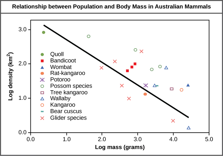
The study of any population usually begins by determining how many individuals of a particular species exist, and how closely associated they are with each other. Within a particular habitat, a population can be characterized by its population size (N), the total number of individuals, and its population density, the number of individuals within a specific area or volume. Population size and density are the two main characteristics used to describe and understand populations. For example, populations with more individuals may be more stable than smaller populations based on their genetic variability, and thus their potential to adapt to the environment. Alternatively, a member of a population with low population density (more spread out in the habitat), might have more difficulty finding a mate to reproduce compared to a population of higher density. As is shown in Figure 45.2, smaller organisms tend to be more densely distributed than larger organisms.
Visual Connection
Population Research Methods
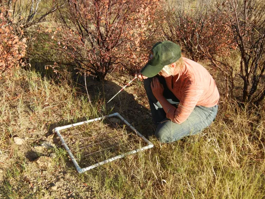
The most accurate way to determine population size is to simply count all of the individuals within the habitat. However, this method is often not logistically or economically feasible, especially when studying large habitats. Thus, scientists usually study populations by sampling a representative portion of each habitat and using this data to make inferences about the habitat as a whole. A variety of methods can be used to sample populations to determine their size and density. For immobile organisms such as plants, or for very small and slow-moving organisms, a quadrat may be used (Figure 45.3). A quadrat is a way of marking off square areas within a habitat, either by staking out an area with sticks and string, or by the use of a wood, plastic, or metal square placed on the ground. After setting the quadrats, researchers then count the number of individuals that lie within their boundaries. Multiple quadrat samples are performed throughout the habitat at several random locations to estimate the population size and density within the entire habitat. The number and size of quadrat samples depends on the type of organisms under study and other factors, including the density of the organism. For example, if sampling daffodils, a 1 m2 quadrat might be used. With giant redwoods, on the other hand, a larger quadrat of 100 m2 might be employed. This ensures that enough individuals of the species are counted to get an accurate sample that correlates with the habitat, including areas not sampled.
For mobile organisms, such as mammals, birds, or fish, scientists use a technique called mark and recapture. This method involves marking a sample of captured animals in some way (such as tags, bands, paint, or other body markings), and then releasing them back into the environment to allow them to mix with the rest of the population. Later, researchers collect a new sample, including some individuals that are marked (recaptures) and some individuals that are unmarked (Figure 45.4). Using the ratio of marked and unmarked individuals, scientists determine how many individuals are in the sample. From this, calculations are used to estimate the total population size.
Species Distribution
In addition to measuring simple density, further information about a population can be obtained by looking at the distribution of the individuals. Species dispersion patterns (or distribution patterns) show the spatial relationship between members of a population within a habitat at a particular point in time. In other words, they show whether members of the species live close together or far apart, and what patterns are evident when they are spaced apart.
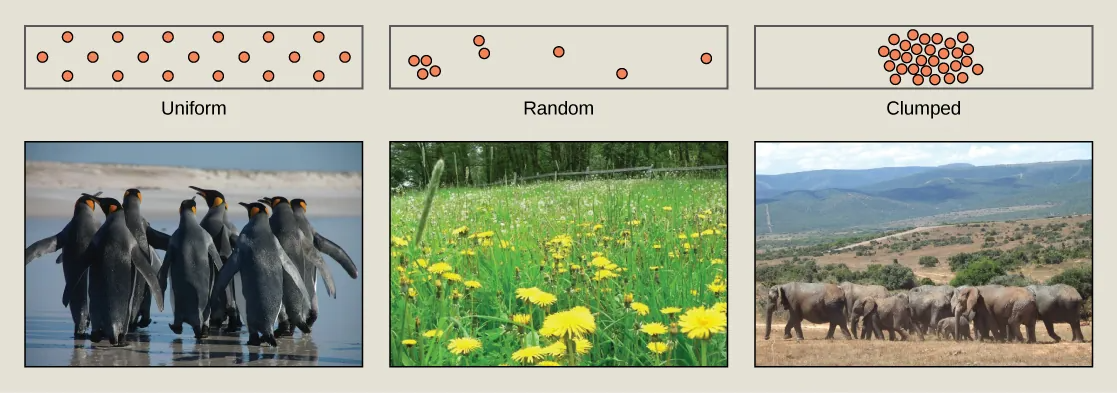
Individuals in a population can be equally spaced apart, dispersed randomly with no predictable pattern, or clustered in groups. These are known as uniform, random, and clumped dispersion patterns, respectively (Figure 45.5). Uniform dispersion is observed in plants that secrete substances inhibiting the growth of nearby individuals (such as the release of toxic chemicals by the sage plant Salvia leucophylla, a phenomenon called allelopathy) and in animals like the penguin that maintain a defined territory. An example of random dispersion occurs with dandelion and other plants that have wind-dispersed seeds that germinate wherever they happen to fall in a favorable environment. A clumped dispersion may be seen in plants that drop their seeds straight to the ground, such as oak trees, or in animals that live in groups (schools of fish or herds of elephants). Clumped dispersions may also be a function of habitat heterogeneity. Thus, the dispersion of the individuals within a population provides more information about how they interact with each other than does a simple density measurement. Just as lower density species might have more difficulty finding a mate, solitary species with a random distribution might have a similar difficulty when compared to social species clumped together in groups.
Demography
While population size and density describe a population at one particular point in time, scientists must use demography to study the dynamics of a population. Demography is the statistical study of population changes over time: birth rates, death rates, and life expectancies. Each of these measures, especially birth rates, may be affected by the population characteristics described above. For example, a large population size results in a higher birth rate because more potentially reproductive individuals are present. In contrast, a large population size can also result in a higher death rate because of competition, disease, and the accumulation of waste. Similarly, a higher population density or a clumped dispersion pattern results in more potential reproductive encounters between individuals, which can increase birth rate. Lastly, a female-biased sex ratio (the ratio of males to females) or age structure (the proportion of population members at specific age ranges) composed of many individuals of reproductive age can increase birth rates.
In addition, the demographic characteristics of a population can influence how the population grows or declines over time. If birth and death rates are equal, the population remains stable. However, the population size will increase if birth rates exceed death rates; the population will decrease if birth rates are less than death rates. Life expectancy is another important factor; the length of time individuals remain in the population impacts local resources, reproduction, and the overall health of the population.
Survivorship Curves
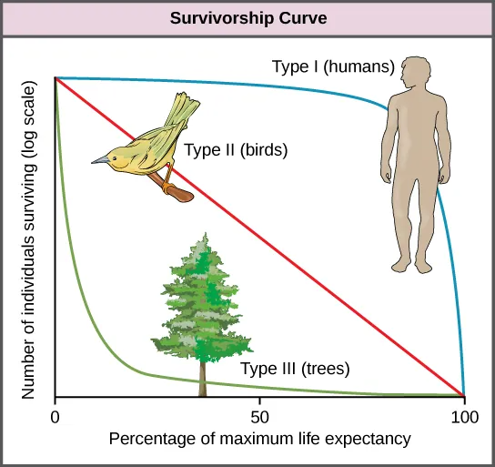
A tool used by population ecologists is a survivorship curve, which is a graph of the number of individuals surviving at each age interval plotted versus time. These curves allow us to compare the life histories of different populations (Figure 45.6). Humans and most primates exhibit a Type I survivorship curve because a high percentage of offspring survive their early and middle years—death occurs predominantly in older individuals. These types of species usually have small numbers of offspring at one time, and they give a high amount of parental care to them to ensure their survival. Birds are an example of an intermediate or Type II survivorship curve because birds die more or less equally at each age interval. These organisms also may have relatively few offspring and provide significant parental care. Trees, marine invertebrates, and most fishes exhibit a Type III survivorship curve because very few of these organisms survive their younger years; however, those that make it to an old age are more likely to survive for a relatively long period of time. Organisms in this category usually have a very large number of offspring, but once they are born, little parental care is provided. Thus these offspring are “on their own” and vulnerable to predation, but their sheer numbers assure the survival of enough individuals to perpetuate the species.
Life Histories
Learning Outcomes
- Describe how life history patterns are influenced by natural selection
- Explain different life history patterns and how different reproductive strategies affect species’ survival
A species’ life history describes the series of events over its lifetime, such as how resources are allocated for growth, maintenance, and reproduction. A species’ life history is genetically determined and shaped by the environment and natural selection.
Life History Patterns and Energy Budgets
Energy is required by all living organisms for their growth, maintenance, and reproduction; at the same time, energy is often a major limiting factor in determining an organism’s survival. Plants, for example, acquire energy from the sun via photosynthesis, but must expend this energy to grow, maintain health, and produce energy-rich seeds to produce the next generation. Animals have the additional burden of using some of their energy reserves to acquire food. Furthermore, some animals must expend energy caring for their offspring. Thus, all species have an energy budget: they must balance energy intake with their use of energy for metabolism, reproduction, parental care, and energy storage (such as bears building up body fat for winter hibernation).
Parental Care and Fecundity
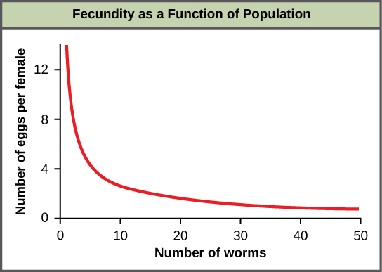
Fecundity is the potential reproductive capacity of an individual within a population. In other words, fecundity describes how many offspring could ideally be produced if an individual has as many offspring as possible, repeating the reproductive cycle as soon as possible after the birth of the offspring. In animals, fecundity is inversely related to the amount of parental care given to an individual offspring. Species, such as many marine invertebrates, that produce many offspring usually provide little if any care for the offspring (they would not have the energy or the ability to do so anyway). Most of their energy budget is used to produce many tiny offspring. Animals with this strategy are often self-sufficient at a very early age. This is because of the energy tradeoff these organisms have made to maximize their evolutionary fitness. Because their energy is used for producing offspring instead of parental care, it makes sense that these offspring have some ability to be able to move within their environment and find food and perhaps shelter. Even with these abilities, their small size makes them extremely vulnerable to predation, so the production of many offspring allows enough of them to survive to maintain the species.
Animal species that have few offspring during a reproductive event usually give extensive parental care, devoting much of their energy budget to these activities, sometimes at the expense of their own health. This is the case with many mammals, such as humans, kangaroos, and pandas. The offspring of these species are relatively helpless at birth and need to develop before they achieve self-sufficiency.
Plants with low fecundity produce few energy-rich seeds (such as coconuts and chestnuts) with each having a good chance to germinate into a new organism; plants with high fecundity usually have many small, energy-poor seeds (like orchids) that have a relatively poor chance of surviving. Although it may seem that coconuts and chestnuts have a better chance of surviving, the energy tradeoff of the orchid is also very effective. It is a matter of where the energy is used, for large numbers of seeds or for fewer seeds with more energy.
Early versus Late Reproduction
The timing of reproduction in a life history also affects species survival. Organisms that reproduce at an early age have a greater chance of producing offspring, but this is usually at the expense of their growth and the maintenance of their health. Conversely, organisms that start reproducing later in life often have greater fecundity or are better able to provide parental care, but they risk that they will not survive to reproductive age. Examples of this can be seen in fishes. Small fish, like guppies, use their energy to reproduce rapidly, but never attain the size that would give them defense against some predators. Larger fish, like the bluegill or shark, use their energy to attain a large size, but do so with the risk that they will die before they can reproduce or at least reproduce to their maximum. These different energy strategies and tradeoffs are key to understanding the evolution of each species as it maximizes its fitness and fills its niche. In terms of energy budgeting, some species “blow it all” and use up most of their energy reserves to reproduce early before they die. Other species delay having reproduction to become stronger, more experienced individuals and to make sure that they are strong enough to provide parental care if necessary.
Single versus Multiple Reproductive Events
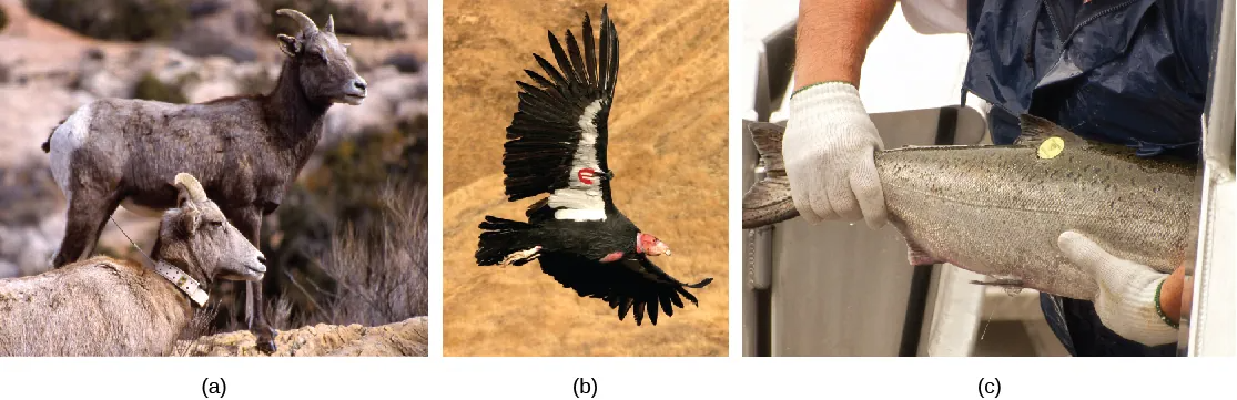
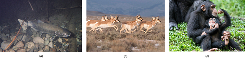
Some life history traits, such as fecundity, timing of reproduction, and parental care, can be grouped together into general strategies that are used by multiple species. Semelparity occurs when a species reproduces only once during its lifetime and then dies. Such species use most of their resource budget during a single reproductive event, sacrificing their health to the point that they do not survive. Examples of semelparity are bamboo, which flowers once and then dies, and the Chinook salmon (Figure 45.7a), which uses most of its energy reserves to migrate from the ocean to its freshwater nesting area, where it reproduces and then dies. Scientists have posited alternate explanations for the evolutionary advantage of the Chinook’s post-reproduction death: a programmed suicide caused by a massive release of corticosteroid hormones, presumably so the parents can become food for the offspring, or simple exhaustion caused by the energy demands of reproduction; these are still being debated.
Iteroparity describes species that reproduce repeatedly during their lives. Some animals are able to mate only once per year, but survive multiple mating seasons. The pronghorn antelope is an example of an animal that goes into a seasonal estrus cycle (“heat”): a hormonally induced physiological condition preparing the body for successful mating (Figure 45.7b). Females of these species mate only during the estrus phase of the cycle. A different pattern is observed in primates, including humans and chimpanzees, which may attempt reproduction at any time during their reproductive years, even though their menstrual cycles make pregnancy likely only a few days per month during ovulation (Figure 45.7c).
Link to Learning
Play this interactive PBS evolution-based mating game to learn more about reproductive strategies.
Population Growth Models
Learning Objectives
- Explain the characteristics of and differences between exponential and logistic growth patterns
- Describe how natural selection and environmental adaptation led to the evolution of particular life history patterns
Although life histories describe the way many characteristics of a population (such as their age structure) change over time in a general way, population ecologists make use of a variety of methods to model population dynamics mathematically. These more precise models can then be used to accurately describe changes occurring in a population and better predict future changes. Certain long-accepted models are now being modified or even abandoned due to their lack of predictive ability, and scholars strive to create effective new models.
Exponential Growth
Charles Darwin, in his theory of natural selection, was greatly influenced by the English clergyman Thomas Malthus. Malthus published a book in 1798 stating that populations with unlimited natural resources grow very rapidly, and then population growth decreases as resources become depleted. This accelerating pattern of increasing population size is called exponential growth.
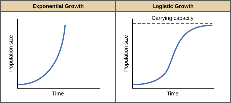
The best example of exponential growth is seen in bacteria. Bacteria reproduce by prokaryotic fission. This division takes about an hour for many bacterial species. If 1000 bacteria are placed in a large flask with an unlimited supply of nutrients (so the nutrients will not become depleted), after an hour, there is one round of division and each organism divides, resulting in 2000 organisms—an increase of 1000. In another hour, each of the 2000 organisms will double, producing 4000, an increase of 2000 organisms. After the third hour, there should be 8000 bacteria in the flask, an increase of 4000 organisms. The important concept of exponential growth is the accelerating population growth rate—the number of organisms added in each reproductive generation—that is, it is increasing at a greater and greater rate. After 1 day and 24 of these cycles, the population would have increased from 1000 to more than 16 billion. When the population size, N, is plotted over time, a J-shaped growth curve is produced (Figure 45.9). The bacteria example is not representative of the real world though where resources are limited. Furthermore, some bacteria will die during the experiment and thus not reproduce, lowering the growth rate.
Logistic Growth
Exponential growth is possible only when infinite natural resources are available; this is not the case in the real world. Charles Darwin recognized this fact in his description of the “struggle for existence,” which states that individuals will compete (with members of their own or other species) for limited resources. The successful ones will survive to pass on their own characteristics and traits (which we know now are transferred by genes) to the next generation at a greater rate (natural selection). To model the reality of limited resources, population ecologists developed the logistic growth model.
Carrying Capacity and the Logistic Model
In the real world, with its limited resources, exponential growth cannot continue indefinitely. Exponential growth may occur in environments where there are few individuals and plentiful resources, but when the number of individuals gets large enough, resources will be depleted, slowing the growth rate. Eventually, the growth rate will plateau or level off (Figure 45.9). This population size, which represents the maximum population size that a particular environment can support, is called the carrying capacity, or K.
A graph of this equation yields an S-shaped curve (Figure 45.9), and it is a more realistic model of population growth than exponential growth. There are three different sections to an S-shaped curve. Initially, growth is exponential because there are few individuals and ample resources available. Then, as resources begin to become limited, the growth rate decreases. Finally, growth levels off at the carrying capacity of the environment, with little change in population size over time.
Role of Intraspecific Competition
The logistic model assumes that every individual within a population will have equal access to resources and, thus, an equal chance for survival. For plants, the amount of water, sunlight, nutrients, and the space to grow are the important resources, whereas in animals, important resources include food, water, shelter, nesting space, and mates.
In the real world, phenotypic variation among individuals within a population means that some individuals will be better adapted to their environment than others. The resulting competition between population members of the same species for resources is termed intraspecific competition (intra- = “within”; -specific = “species”). Intraspecific competition for resources may not affect populations that are well below their carrying capacity—resources are plentiful and all individuals can obtain what they need. However, as population size increases, this competition intensifies. In addition, the accumulation of waste products can reduce an environment’s carrying capacity.
Carrying Capacity
Learning Objectives
- Give examples of how the carrying capacity of a habitat may change
- Compare and contrast density-dependent growth regulation and density-independent growth regulation, giving examples
- Describe how natural selection and environmental adaptation leads to the evolution of particular life-history patterns
The logistic model of population growth, while valid in many natural populations and a useful model, is a simplification of real-world population dynamics. Implicit in the model is that the carrying capacity of the environment does not change, which is not the case. The carrying capacity varies annually: for example, some summers are hot and dry whereas others are cold and wet. In many areas, the carrying capacity during the winter is much lower than it is during the summer. Also, natural events such as earthquakes, volcanoes, and fires can alter an environment and hence its carrying capacity. Additionally, populations do not usually exist in isolation. They engage in interspecific competition: that is, they share the environment with other species competing for the same resources. These factors are also important to understanding how a specific population will grow.
Nature regulates population growth in a variety of ways. These are grouped into density-dependent factors, in which the density of the population at a given time affects growth rate and mortality, and density-independent factors, which influence mortality in a population regardless of population density. Note that in the former, the effect of the factor on the population depends on the density of the population at onset. Conservation biologists want to understand both types because this helps them manage populations and prevent extinction or overpopulation.
Density-Dependent Regulation
Most density-dependent factors are biological in nature (biotic), and include predation, inter– and intraspecific competition, accumulation of waste, and diseases such as those caused by parasites. Usually, the denser a population is, the greater its mortality rate. For example, during intra- and interspecific competition, the reproductive rates of the individuals will usually be lower, reducing their population’s rate of growth. In addition, low prey density increases the mortality of its predator because it has more difficulty locating its food source.
Density-Independent Regulation and Interaction with Density-Dependent Factors
Many factors, typically physical or chemical in nature (abiotic), influence the mortality of a population regardless of its density, including weather, natural disasters, and pollution. An individual deer may be killed in a forest fire regardless of how many deer happen to be in that area. Its chances of survival are the same whether the population density is high or low. The same holds true for cold winter weather.
In real-life situations, population regulation is very complicated and density-dependent and independent factors can interact. A dense population that is reduced in a density-independent manner by some environmental factor(s) will be able to recover differently than a sparse population. For example, a population of deer affected by a harsh winter will recover faster if there are more deer remaining to reproduce.
Life Histories of K-selected and r-selected Species
While reproductive strategies play a key role in life histories, they do not account for important factors like limited resources and competition. The regulation of population growth by these factors can be used to introduce a classical concept in population biology, that of K-selected versus r-selected species.
The concept relates to a species’ reproductive strategies, habitat, and behavior, especially in the way that they obtain resources and care for their young. It includes length of life and survivorship factors as well. Population biologists have grouped species into the two large categories—K-selected and r-selected—although the categories are really two ends of a continuum.
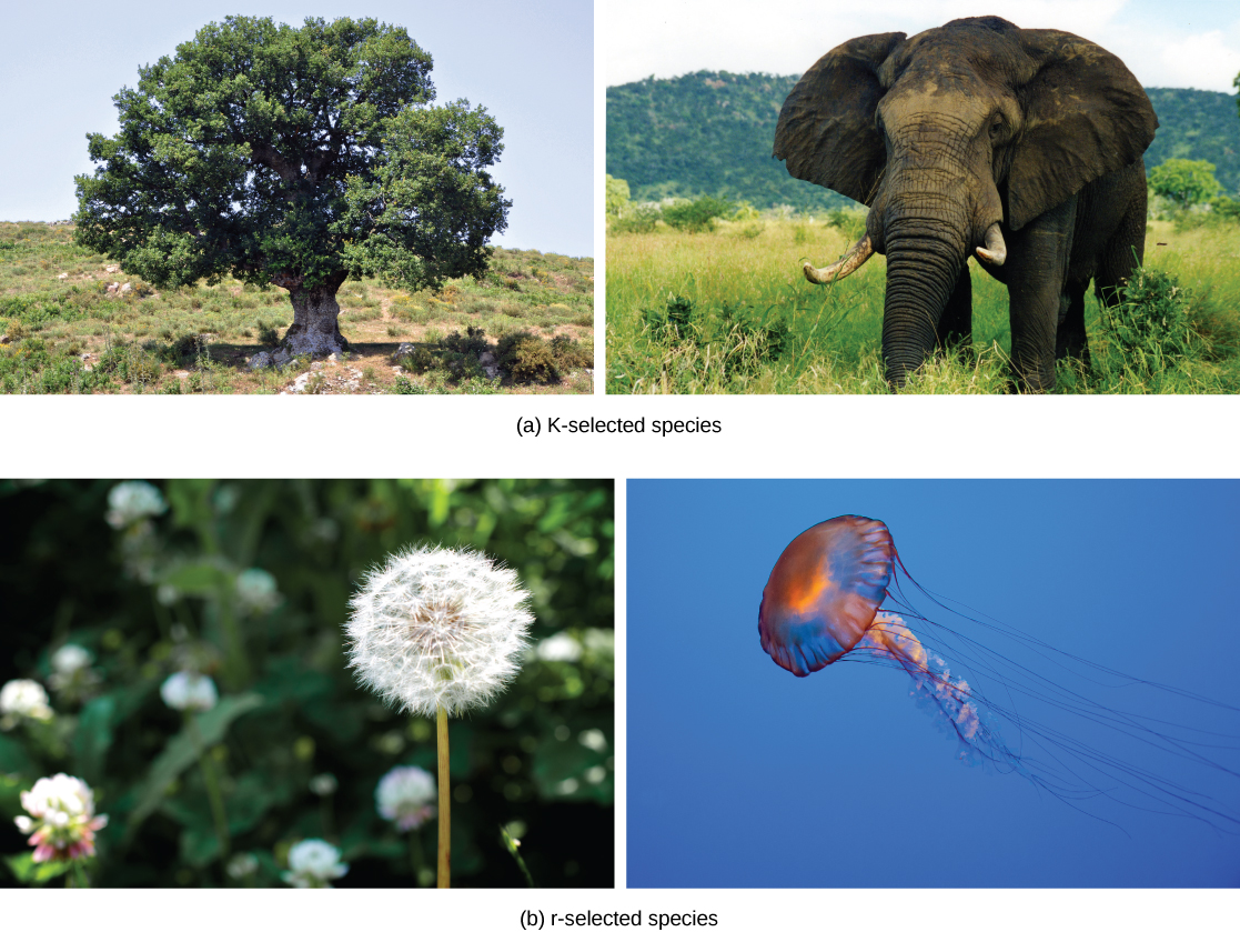
K-selected species are species selected by stable, predictable environments. Populations of K-selected species tend to exist close to their carrying capacity (hence the term K-selected) where intraspecific competition is high. These species have few, large offspring, a long gestation period, and often give long-term care to their offspring (Table 45.2). While larger in size when born, the offspring are relatively helpless and immature at birth. By the time they reach adulthood, they must develop skills to compete for natural resources. In plants, scientists think of parental care more broadly: how long fruit takes to develop or how long it remains on the plant are determining factors in the time to the next reproductive event. Examples of K-selected species are primates (including humans), elephants, and plants such as oak trees (Figure 45.13 a).
In contrast, r-selected species have a large number of small offspring (hence their r designation (Table 45.2). This strategy is often employed in unpredictable or changing environments. Animals that are r-selected do not give long-term parental care and the offspring are relatively mature and self-sufficient at birth. Examples of r-selected species are marine invertebrates, such as jellyfish, and plants, such as the dandelion (Figure 45.13b). Dandelions have small seeds that are wind dispersed long distances. Many seeds are produced simultaneously to ensure that at least some of them reach a hospitable environment. Seeds that land in inhospitable environments have little chance for survival since their seeds are low in energy content. Note that survival is not necessarily a function of energy stored in the seed itself.
Characteristics of K-selected versus r-selected species
| Characteristics of K-selected species | Characteristics of r-selected species |
| Mature late | Mature early |
| Greater longevity | Lower longevity |
| Increased parental care | Decreased parental care |
| Increased competition | Decreased competition |
| Fewer offspring | More offspring |
| Larger offspring | Smaller offspring |
Modern Theories of Life History
By the second half of the twentieth century, the concept of K- and r-selected species was used extensively and successfully to study populations. The r– and K-selection theory, although accepted for decades and used for much groundbreaking research, has now been reconsidered, and many population biologists have abandoned or modified it. Over the years, several studies attempted to confirm the theory, but these attempts have largely failed. Many species were identified that did not follow the theory’s predictions. Furthermore, the theory ignored the age-specific mortality of the populations which scientists now know is very important. New demographic-based models of life history evolution have been developed which incorporate many ecological concepts included in r– and K-selection theory as well as population age structure and mortality factors.
Link to Learning
For a summary of population ecology, watch the Crash Course Biology video “The Texas Mosquito Mystery.” (Don’t worry about the mathematical equations.)
