Particles in an ideal gas all travel at relatively high speeds, but they do not travel at the same speed. The rms speed is one kind of average, but many particles move faster and many move slower. The actual distribution of speeds has several interesting implications for other areas of physics, as we will see in later chapters.

The Maxwell-Boltzmann Distribution

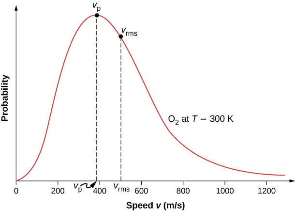
The motion of molecules in a gas is random in magnitude and direction for individual molecules, but a gas of many molecules has a predictable distribution of molecular speeds. This predictable distribution of molecular speeds is known as the Maxwell-Boltzmann distribution, after its originators, who calculated it based on kinetic theory, and it has since been confirmed experimentally (Figure 2.15).

To understand this figure, we must define a distribution function of molecular speeds, since with a finite number of molecules, the probability that a molecule will have exactly a given speed is 0.

We define the distribution function [latex]f(v)[/latex] by saying that the expected number [latex]N(v_1,v_2)[/latex] of particles with speeds between [latex]v_1[/latex] and [latex]v_2[/latex] is given by

[latex]N( v_1 , v_2 ) = N \int_{v_1}^{v_2} f(v)dv .[/latex]

[Since N is dimensionless, the unit of f(v) is seconds per meter.] We can write this equation conveniently in differential form:

[latex]dN = N f(v) dv.[/latex]

In this form, we can understand the equation as saying that the number of molecules with speeds between v and [latex]v + dv[/latex] is the total number of molecules in the sample times f(v) times dv. That is, the probability that a molecule’s speed is between v and v + dv is f(v)dv.

We can now quote Maxwell’s result, although the proof is beyond our scope.

The factors before the [latex]v^2[/latex] are a normalization constant; they make sure that [latex]N( 0,\infty ) = N[/latex] by making sure that [latex]\int_0^\infty f(v)dv = 1[/latex]. Let’s focus on the dependence on v. The factor of [latex]v^2[/latex] means that [latex]f(0)=0[/latex] and for small v, the curve looks like a parabola. The factor of [latex]e^{-m_0v^2/2k_\text{B}T}[/latex] means that [latex]\displaystyle \lim_{v\to{\infty}} f(v) = 0[/latex] and the graph has an exponential tail, which indicates that a few molecules may move at several times the rms speed. The interaction of these factors gives the function the single-peaked shape shown in the figure.

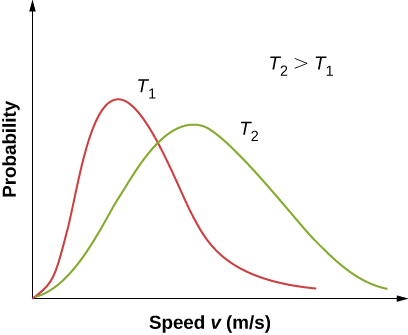
Figure 2.16 shows that the curve is shifted to higher speeds at higher temperatures, with a broader range of speeds.

We can use a probability distribution to calculate average values by multiplying the distribution function by the quantity to be averaged and integrating the product over all possible speeds. (This is analogous to calculating averages of discrete distributions, where you multiply each value by the number of times it occurs, add the results, and divide by the number of values. The integral is analogous to the first two steps, and the normalization is analogous to dividing by the number of values.) Thus the average velocity is

Similarly,

[latex]v_{rms} = \sqrt{\bar{v^2}} = \sqrt{\int_0^\infty v^2 f(v)dv} = \sqrt{\frac{3 k_B T}{m}} = \sqrt{\frac{3RT}{M}}[/latex]

as in Pressure, Temperature, and RMS Speed. The most probable speed, also called the peak speed [latex]v_p[/latex], is the speed at the peak of the velocity distribution. (In statistics it would be called the mode.) It is less than the rms speed [latex]v_\text{rms}[/latex]. The most probable speed can be calculated by the more familiar method of setting the derivative of the distribution function, with respect to v, equal to 0. The result is

which is less than [latex]v_\text{rms}[/latex]. In fact, the rms speed is greater than both the most probable speed and the average speed.

The peak speed provides a sometimes more convenient way to write the Maxwell-Boltzmann distribution function:

In the factor [latex]e^{-mv^2/2k_\text{B}T}[/latex], it is easy to recognize the translational kinetic energy. Thus, that expression is equal to [latex]e^{-K/k_\text{B}T}[/latex]. The distribution f(v) can be transformed into a kinetic energy distribution by requiring that [latex]f(K)dK=f(v)dv[/latex]. Boltzmann showed that the resulting formula is much more generally applicable if we replace the kinetic energy of translation with the total mechanical energy E. Boltzmann’s result is

[latex]f(E) = \frac{2}{\sqrt{\pi}} {( k_B T)}^{-3/2} \sqrt{E} e^{-E/ k_B T} = \frac{2}{\sqrt{\pi} {( k_B T)}^{3/2}}\frac{\sqrt{E}}{e^{E/ k_B T}} .[/latex]

The first part of this equation, with the negative exponential, is the usual way to write it. We give the second part only to remark that [latex]e^{E/k_\text{B}T}[/latex] in the denominator is ubiquitous in quantum as well as classical statistical mechanics.

We can now gain a qualitative understanding of a puzzle about the composition of Earth’s atmosphere. Hydrogen is by far the most common element in the universe, and helium is by far the second-most common. Moreover, helium is constantly produced on Earth by radioactive decay. Why are those elements so rare in our atmosphere? The answer is that gas molecules that reach speeds above Earth’s escape velocity, about 11 km/s, can escape from the atmosphere into space. Because of the lower mass of hydrogen and helium molecules, they move at higher speeds than other gas molecules, such as nitrogen and oxygen. Only a few exceed escape velocity, but far fewer heavier molecules do. Thus, over the billions of years that Earth has existed, far more hydrogen and helium molecules have escaped from the atmosphere than other molecules, and hardly any of either is now present.

We can also now take another look at evaporative cooling, which we discussed in the chapter on temperature and heat. Liquids, like gases, have a distribution of molecular energies. The highest-energy molecules are those that can escape from the intermolecular attractions of the liquid. Thus, when some liquid evaporates, the molecules left behind have a lower average energy, and the liquid has a lower temperature.