Chapter 5: Theory of Airfoil Lift Aerodynamics

mi508668

5 Chapter 5: Theory of Airfoil Lift Aerodynamics

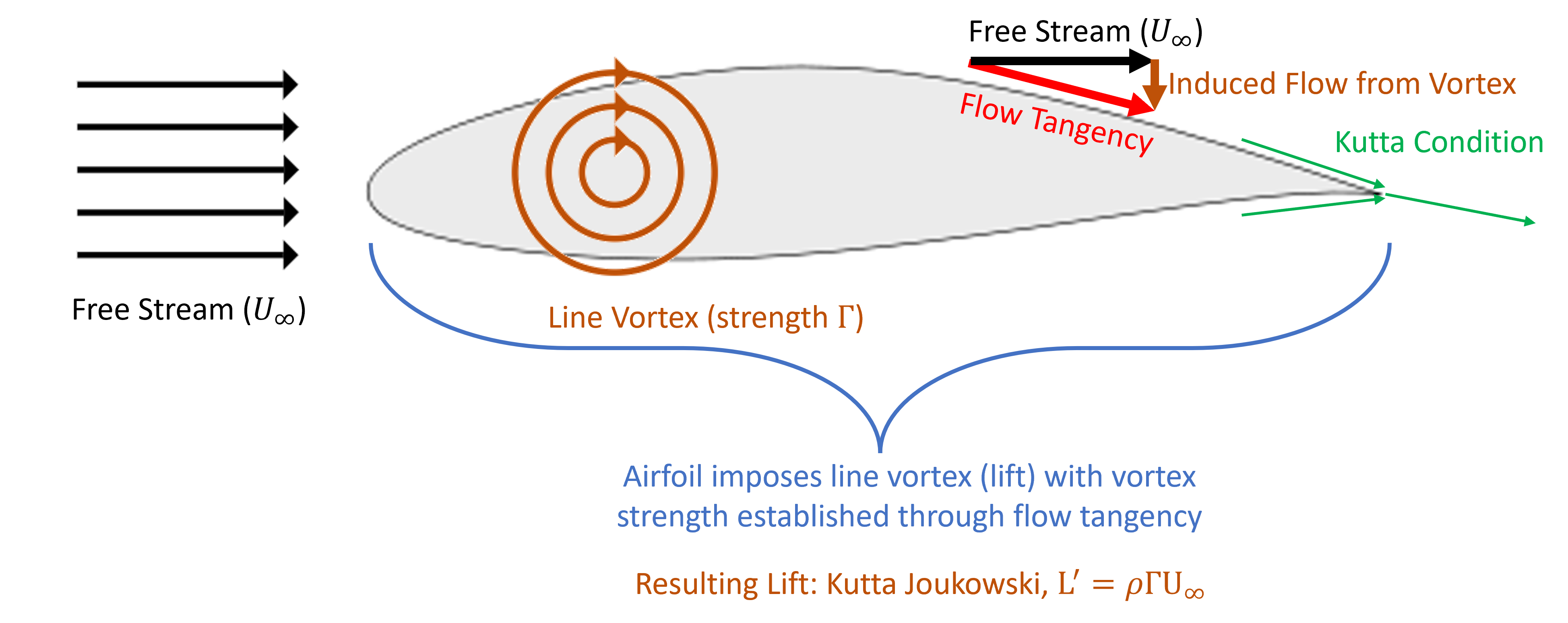
Airfoil theory is largely governed by potential flow theory. Specifically, a key component of airfoil aerodynamics theory is the combination of:

Free-stream velocity elementary flow
Line vortex model elementary flow
Flow tangency
Kutta condition
Kutta-Joukowski theorem

These concepts are depicted in the figure below. Let us review all of these concepts to understand the core theory of airfoil aerodynamics.

Background Theory and Concepts

Airfoil

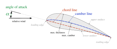
Airfoils are the cross-sections of a wing or lifting surface (i.e., propellers and fins). These shapes drive the underlying performance of a lifting surface. As indicated in the Figure below, the shape is described as the cross-section of the lifting surface. These shapes can vary from a high-drag cylinder, used for support, to low-drag shapes (conventionally thought of as an airfoil) associated with wings and high-speed flight.

Airfoils can be characterized as indicated in the Figure. A few key terms are the angle of attack, $\alpha$ , which is defined as the incidence angle of the chord line with respect to the free-stream velocity. The chordline is the line connecting the leading and trailing edges. The chord length (c) is the length of the chordline and the common lengthscale for airfoils. Then the camberline is defined as the line through the mean thickness of the airfoil. Through these characteristics, airfoils can be generalized.

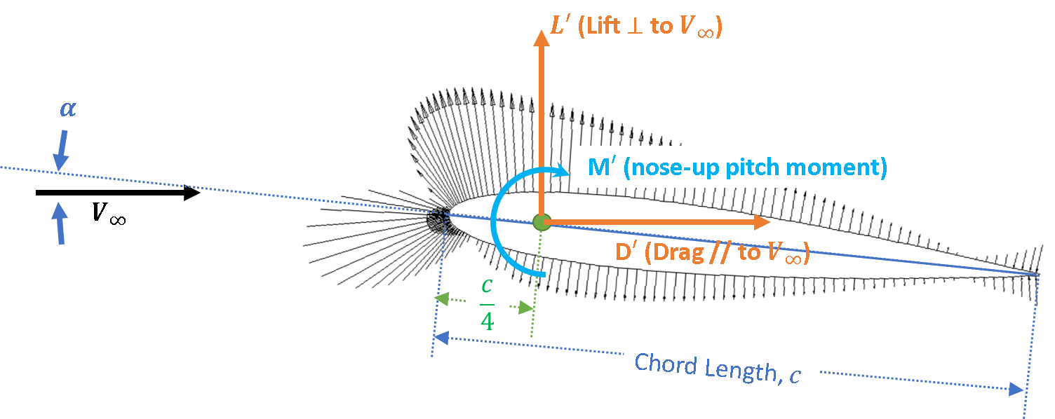
Aerodynamic loads generally include a lift, drag, and pitching moment. These forces, respectively relate to supporting the aircraft, power, and trim (or straight and level flight). The convention to describe these loads are provided in the Figure below.

Description of aerodynamic force convention on an airfoil in terms of lift, drag, and pitching moment.

Baseline Aerodynamic Scaling, Parameters, and Concepts

Aerodynamic scaling and nondimensional numbers are critical to aerodynamics. They enable us to scale loads from one condition to another. In general, aerodynamic forces relate to the integration of pressure. Because of this, it is common to define the dynamic pressure, $q_\infty$ , as

(1) $\begin{equation*} q_\infty=\frac{1}{2}\rho V_\infty^2. \end{equation*}$

This dynamic pressure relates to the overall aerodynamic energy in the flow. Two other critical parameters relate local flow quantities to aerodynamic forces. Recall the momentum equation, given as

(2) $\begin{equation*} \frac{\partial }{\partial t}\iiint_{CV}{\rho \vec{V} dV} + \iint_{CS} {\rho \vec{V} \left(\vec{V}}\cdot\vec{ds}\right)=-\iint_{CS}{pd\vec{s}}+\iint_{CS}{\vec{\tau_w} ds} \end{equation*}$

For aerodynamic forces, we want to focus on the loads on the aerodynamic surfaces themselves. In Fig. 1, we can see the forces on the airfoil are reaction forces to moving the fluid. These are the pressure and viscous forces on the control volume defined on the airfoil surface.

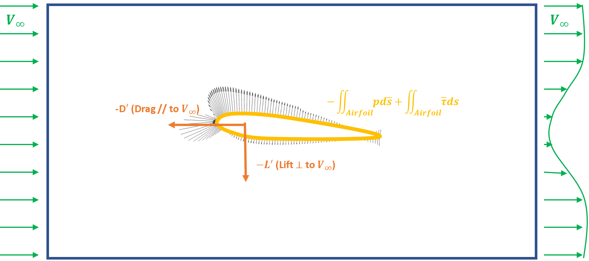
Figure: Control volume for flow over an airfoil in a wind tunnel. Note that airfoil forces are acting on the fluid. The CV integral terms on the surface are the aerodynamic interactions in terms of pressure and shear force.

Aerodynamic forces are reaction forces to the terms on the right-hand side of the equation, integrated over the aerodynamic surface. Note that the pressure/shear forces of the fluid on the airfoil (i.e., the aerodynamic forces) are equal and opposite to the pressure and shear forces the airfoil imposes on the fluid. Hence, the aerodynamic forces (i.e., – of fluid convention) can be described as

(3) $\begin{equation*} \vec{F}=\iint_s{pd\vec{s}}-\iint_s{\vec{\tau_w} ds}. \end{equation*}$

The force coefficients scale as follows

(4) $\begin{equation*} C_F=\frac{F}{q_\infty A}. \end{equation*}$

Here, $A$ is a reference area that is defined specifically to applications or conventions. For example, a wing normally uses planform area while a fuselage may use a projected frontal area. The reference A is really not important, what is important is consistent usage of $A$ . We can then compute a force coefficient as follows:

(5) $\begin{equation*} C_F=\frac{\vec{F}}{q_\infty A}=\frac{\iint_s{pd\vec{s}}}{q_\infty A}-\frac{\iint_s{\vec{\tau_w} ds}}{q_\infty A}. \end{equation*}$

Which can be reduced as follows:

(6) $\begin{equation*} C_F=\frac{\vec{F}}{q_\infty A}=\frac{1}{A}\iint_s{\frac{p}{q_\infty}d\vec{s}}-\frac{1}{A}\iint_s{\frac{\vec{\tau_w}}{q_\infty}ds}. \end{equation*}$

Note that the surface integral of constant pressure, $p_infty$ , is zero (recall from hydrostatics). Hence, $\frac{1}{A}\iint_s{\frac{p_\infty}{q_\infty}d\vec{s}}=0$ . This can be subtracted from Eq. 6, to yield

(7) $\begin{equation*} C_F=\frac{\vec{F}}{q_\infty A}=\frac{1}{A}\iint_s{\frac{p-p_\infty}{q_\infty}d\vec{s}}-\frac{1}{A}\iint_s{\frac{\vec{\tau_w}}{q_\infty}ds}. \end{equation*}$

These terms yield local forces in terms of a local pressure coefficient,

(8) $\begin{equation*} c_p=\frac{p-p_\infty}{q_\infty}, \end{equation*}$

which yields the surface-normal force. We can also obtain the local skin friction coefficient,

(9) $\begin{equation*} c_f=\frac{\tau_w}{q_/infty}, \end{equation*}$

which is a normalized, surface-parallel force from viscous forces.

The underlying flow field drives the pressure and viscous forcing. In the context of aerodynamics, there are two key scaling parameters associated with the flow dynamics. The first is the Reynolds number,

(10) $\begin{equation*} Re=\frac{\rho V_\infty l}{\mu}=\frac{Inertial\;Forces}{Viscous\;Forces}. \end{equation*}$

Conceptually, $Re$ defines how important viscous forces are with respect to the inertia of the flow. Here, density, $\rho$ , free-stream velocity, $V_\infty$ , a length scale (typically chord), $l$ , and dynamic viscosity, $\mu$ , all relate to this nondimensional number.

The second key driving fluid scale is the Mach number,

(11) $\begin{equation*} M=\frac{V_\infty}{a}=\frac{Speed\;Of\;Vehicle}{Speed\;Of\;Sound\;(Disturbance\;Speed)}. \end{equation*}$

Conceptually, $M$ relates to the speed of a vehicle in comparison to how fast pressure waves move. These two parameters govern kinematic similarity in fluid dynamics, which drive pressure and viscous forces, which ultimately relate to the aerodynamic force response.

Kutta condition

Simple in concept and critical (despite ad-hoc) component to aerodynamics. At its core, the Kutta condition implies either a smooth flow at the trailing edge of an airfoil or a stagnation point at the trailing edge. Conventional wisdom has in the past implied that the Kutta condition is a “viscous patch” that ties potential flow to a physical condition.

Alternatively, a recent theory derived based on variational theory was developed arguing that rather than a viscous patch, Kutta condition is essentially a result of the incorporation of the momentum equation (recall that the momentum equation is only used for pressure). The authors describe this physical as discussed by Gonzalez and Taha (2022):

“In words, lift is due to (i) momentum conservation, (ii) continuity (the fluid has to fill the given space), and (iii) the body’s hard constraint (i.e. presence of the body inside the fluid), which forces the flow to move around the body without creating void to maintain (ii).”

Regardless, Kutta condition is a physical observation that is used to fix a potential flow solution based on the conservation of mass to a physical condition relevant to airfoils. It is typically done by enforcing one of two conditions at the airfoil trailing edge: (1) a stagnation point, or (2) no lift production (or circulation).

Kutta-Joukowski Theorem:

The concept of the Kutta-Joukowski Theorom drives a correlation between the lift per unit span to be directly proportional to the circulation around the body. Specifically, it states that

(12) $\begin{equation*} L'=\rho\Gamma U_\infty \end{equation*}$

where $L'$ is the lift per unit span, $rho$ is the fluid velocity, $\Gamma$ is the circulation, and $U_\infty$ is the free stream velocity. Recall that circulation is defined as

(13) $\begin{equation*} \Gamma =\oint \bar{V}\cdot d\bar{s}. \end{equation*}$

Where (+) is in the clockwise direction. What does this mean? First, let’s recall that a flow with Circulation is not the same as a flow with rotation. Rotational flows are described by viscous forces and imply the fluid elements rotate, see for example this link. In the later example in the link are two flows that both have circulation (as the flows rotate like a tornado, hurricane, or vortex), but only one is rotational (where the fluid elements themselves rotate). Circulation is a feature relevant to vortices, and via Kutta-Jukowski, is why line-vortices are critical for lift generaton in potential flow.

Examples: Kutta Joukowski Thoerom Derviation

Thin Airfoil Models of Aerodynamics

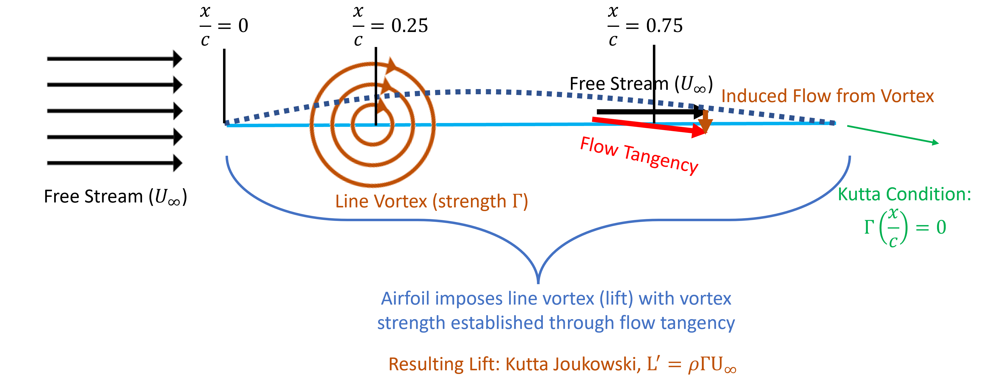
Now let’s explore thin airfoil models. The concept is depicted below. Note the distinct difference between our panel code and the model depicted in the first Figure. That is, the airfoil is treated to have no thickness and approximately look like a camberline. At the camberline, flow tangency is enforced which implies that the line vortex strength is established through satisfying flow tangency on the camberline. This model drives the basics of airfoil theory and will be explored in the context of (1) thin-airfoil theory, (2) numerical thin-airfoil theory, and (3) Wiessinger’s approximation. Normally theory is introduced in this order, but let’s flip the ordering to gradually bring in more complex concepts.

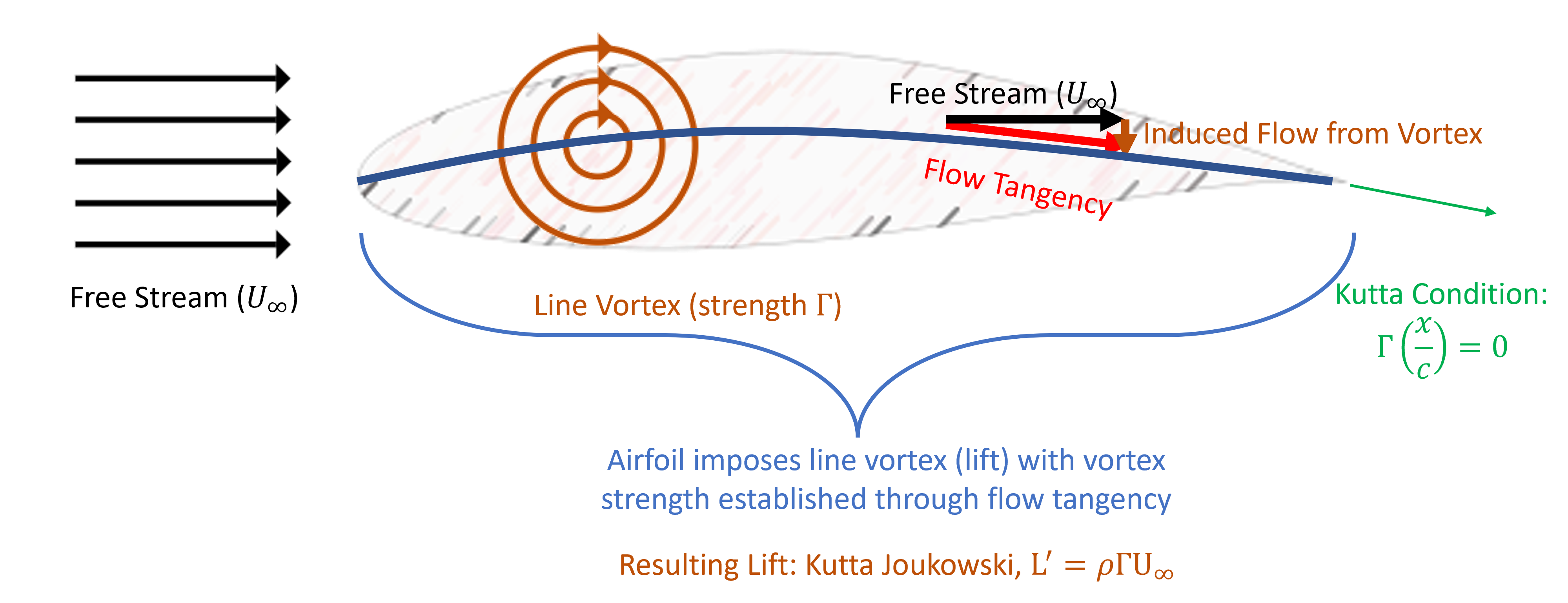
Figure: Thin airfoil model where airfoil approximately has no thickness. Note that this omits a small angle assumption that treats camber on chordline.

Wiessinger’s approximation

Wiessinger’s approximation is a simplified form of TAT. The overall model is described in the Figure below. Note that compared to the previous model, the line vortex is positioned at the quarter chord and on the chordline. The line vortex induces a velocity as follows
begin{equation}
v_theta=frac{Gamma}{2pi r}.
end{equation}
As indicated in the flow tangency constraint, this induced velocity is evaluated only at the 3/4 chord location and on the chordline (with the slope of the camberline). Note that positioning on the chordline (rather than the camberline) is consistent with a small angle assumption (i.e., $cos{alpha}approx 1.0$ and $sin{alpha}approx alpha$ ). This certainly causes some confusion, but simplifies the math and is not essentially to understanding the model. The model ultimately solves for the vortex strength, $\Gamma$ , that yeilds lift through Kutta-Joukowski Th. (Eq. (ref{eq:KuttaJouk})) using this value of $\Gamma$ .

Weissinger’s approximation is much more physically intuitive than the formal thin airfoil theory, so please focus to understand and master this first. The result of this model is a very flexible and is rather simple model of airfoil lift aerodynamics. The model is also extendable to the aerodynamics of a cambered airfoil, flapped airfoils, and airfoils operating together. A sample of its application is provided in the video below.

Examples: Development of Wiessinger’s approximation

Numerical Thin-Airfoil Theory

Now consider expanding Wiessinger’s approximation into many elements that represent the airfoil camberline in detail. This approach is referred to as numerical thin-airfoil theory (and is the discretized representation of formal thin-airfoil theory). The overall model is described in the Figure below. There the extension of Weissinger’s approximation should be seen, that is, we basically break the camber line into individual segments ( $j$ ) indicated by the purple sections. In this case, we discretize the camberline into $N_p$ -chordal sections. Each of these sections has a length $\Delta s_j$ and is composed of a line vortex with strength $\gamma_j$ at its 1/4 length, while flow tangency is enforced at its 3/4 length. And, similar to Wiessinger’s approximation, the camberline slope is projecting to the chordline. We can then see the final Numerical thin-airfoil theory (TAT) model composed of N-line vortices with N-flow tangency conditions. Similar to the panel code, this develops an NxN algebraic and linear system that is solveable.

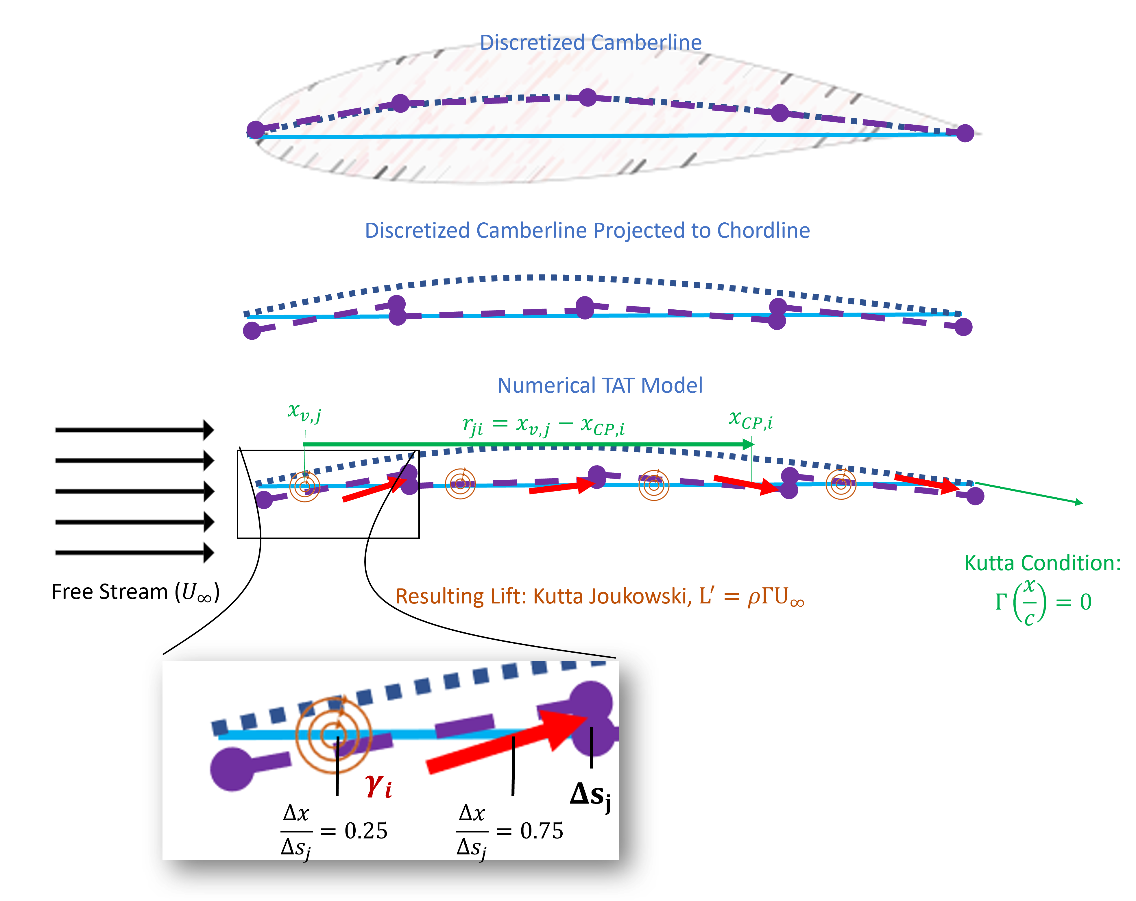
Let’s dig a little deeper into how we would solve this. As indicated in the blowup in the figure above, each panel has a line-vortex and corresponding strength. Each of these vortices induces a flow on each of the panels.The general equation for an induced velocity induced by a line vortex is given as

(14) $\begin{equation*} v_\theta=\frac{\gamma}{2\pi r} \end{equation*}$

To generalize into the model above, we can describe an induced velocity ( $w_{i,j}$ ) which is normal to the chordline by the vortex on panel $j$ onto panel $i$ . The formal extension is given as:

(15) $\begin{equation*} \left. \frac{dz}{dx}\right|_j=\frac{w}{u}=\frac{w_{\infty}+\sum_{j=1}^{N_p} w_{i,j}}{u_{\infty}}. \end{equation*}$

Here, the induced velocity from panel $j$ onto control point $i$ is given as

(16) $\begin{equation*} w_{i,j}=\frac{\gamma_j \Delta s_j}{2\pi \left(x_{v,j}-x_{CP,i} \right )}. \end{equation*}$

Recall, $\gamma$ is positive for a clockwise direction, $r_{j,i}$ is the distance from the vortex position on section $j$ to the flow tangency point on section $i$ . Hence, the sign flips depending on if $j$ is upstream or downstream of $i$ . The diagram below indicates the model formulation from the induced flow from the 3rd panel ( $j=3$ ). Note that the induced flow is downwards on the downstream panels, and upwards on the upstream panels.

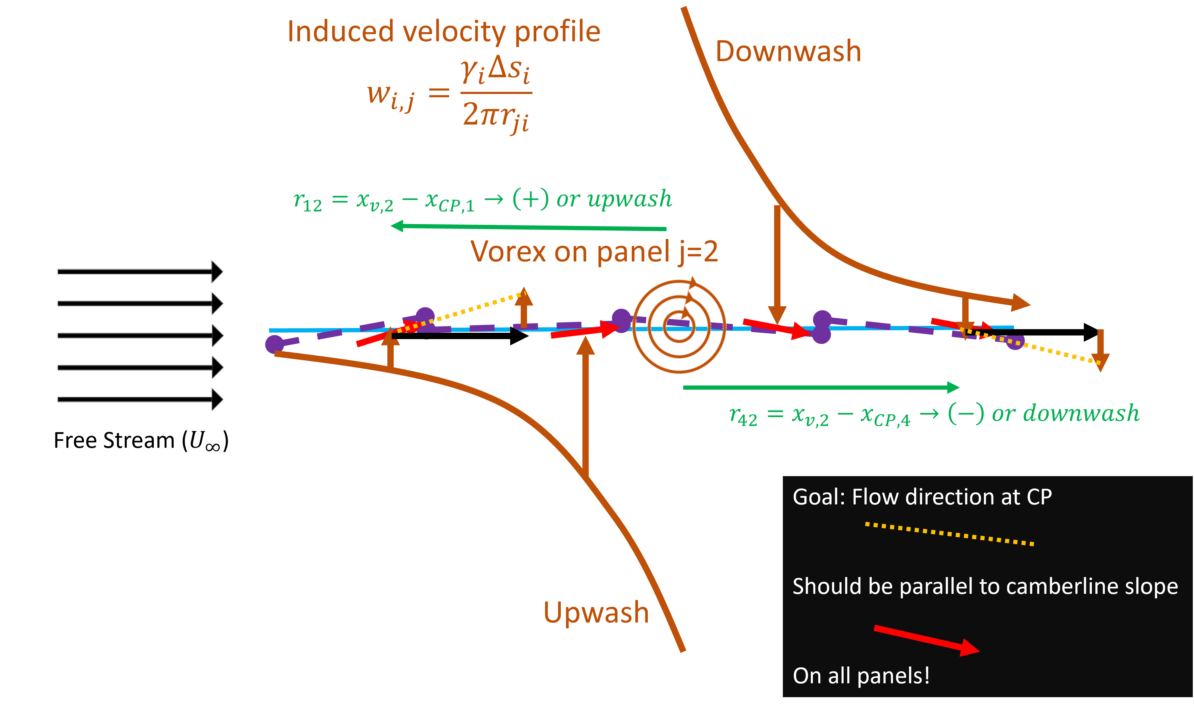
Figure: Diagram showing the induced flow profile induced onto all segments induced from segment 2 (j=2).

In this entire process, remember, we are utilizing an underlying assumption that flow tangency is enforced on the chordline. Without this assumption, there is a demand to expand the analysis to directions that are not chord normal which is much more complex. Ultimately we build a potential flow solution for velocity such that it is given by the free stream + all the contributions from each of the $N_P$ sections, which is given as

(17) $\begin{equation*} {\bar{V}}={\bar{V}}_\infty+\bar{k}\left[\sum_{j=1}^{N_P}\frac{\gamma_j\Delta s_j}{2\pi \left(x_{v,j}-x_{CP,i}\right)}\right]. \end{equation*}$

Here, $\bar{V}=u\bar{i}+w\bar{k}$ . We then satisfy flow tangency at each control point via

(18) $\begin{equation*} \left. \frac{dz}{dx}\right|_j=\frac{w}{u}=\frac{w_{\infty}+w_i}{u_{infty}}=\frac{w}{u}, \end{equation*}$

which is a constraint that states that the slope of the camberline is equal to the slope of the velocity.

Perhaps the best path to understanding the theory involves working through a stepwise procedure as given below:
Step 1: Define the BCs

Free stream flight condition
(19) $\begin{equation*} \bar V_\infty=u_\infty\bar{i}+w_\infty \bar{j} \end{equation*}$
Airfoil discretization which demands (for all $N_p$ ) dividing the camberline into segments. Segment $i$ is formed between two points on the camberline: (1) the starting point $\left(x_{e,i},z_{e,i}\right)$ , and (2) the endpoint $\left(x_{e,i+1},z_{e,i+1}\right)$ . Note that this needs to be done for all segments.
Airfoil shape which demands (for all $N_p$ ) by defining the slope for segment $i$ as

(20) $\begin{equation*} \left. \frac{dz}{dx}\right|_j=\frac{z_{e,i+1}-z_{e,i}}{x_{e,i+1}-x_{e,i}} \end{equation*}$

Step 2: Compute the control points

Line vortex points are (1/4 length of each panel). Use the edge points ( $x_{e,j}$ ) of each section:
(21) $\begin{equation*} x_{v,j}=0.25\left(x_{e,j+1}-x_{e,j}\right) \end{equation*}$
Flow tangency points are (3/4 length of each panel)
(22) $\begin{equation*} x_{cp,j}=0.75\left(x_{e,j+1}-x_{e,j}\right) \end{equation*}$

Why are $x_v$ and $x_{cp}$ not collocated? What happens to the induced velocity at $x_v$ ? Why can we not handle this numerically?

Step 3: Compute the panel length and slope or normal vector
Provides a scaling of the overall strength. Here, $\gamma$ is per-unit length, hence it is important to think of these as “finite” source sheet segments that are assessed at the quarter chord. The source sheet size can be computed as:

(23) $\begin{equation*} \Delta s_{j}=\left(x_{e,j+1}-x_{e,j}\right) \end{equation*}$

Step 4: Now compute the influence coefficients
This is where the discussion of Eqn (15) is involved. Here, these induced velocities are solved to (as a group of all segments) satisfy flow tangency which forms a linear algebraic system of equations. These equations are therefore used to form coefficients for an $A$ matrix. Recall from Eqn (15) that $\gamma$ is positive for a clockwise direction hence, then $r_{ji}$ (the vector from the control point at $j$ to the vortex point $i$ ) is positive, the induced flow is downwards $-z$ . When the sign flips, ie, the control point is upstream of the vortex, the induced velocity is upwards ( $+z$ ). Flow tangency is obtained by the requirement that:

(24) $\begin{equation*} \left. \frac{dz}{dx}\right|_j=\frac{w}{u}=\frac{w_{\infty}+\sum_{j=1}^{N_p} w_{i,j}}{u_{\infty}} \end{equation*}$

We can rearrange to obtain:

(25) $\begin{equation*} u_\infty \left. \frac{dz}{dx}\right|_j -w_\infty =\sum_{j=1}^{N_p} w_{i,j} \end{equation*}$

Our A matrix elements come from the right-hand side of Eq. (ref{eq:linSys}). Specifically, each element can be described as

(26) $\begin{equation*} A_{i,j}=\frac{w_{i,j}}{\gamma_j}=\frac{\Delta s_j}{2\pi \left(x_{v,j}-x_{CP,i} \right )} \end{equation*}$

Our x vector elements represent the strengh of the vortex sheet segment, which

(27) $\begin{equation*} x_j=\gamma_j. \end{equation*}$

Finally, our $b$ matrix elements come from enforcing flow tangency, from Eq. (25) this is

(28) $\begin{equation*} b_j=u_\infty \left. \frac{dz}{dx}\right|_j -w_\infty. \end{equation*}$

Recall the approximations and be sure to keep these in mind when utilizing the method/model.

Step 5: Solve for x (or the $\gamma$ s)

This step involves utilizing an algorithm to solve the linear system, recall Guass-Siedel, iterative methods, etc. Here we just assume we have software that can provide this for us as follows

(29) $\begin{equation*} x=A^{-1}b. \end{equation*}$

Step 6:Compute the Load
The last step involves extracting the aerodynamic lift. Rather than force integration, here we utilize the Kutta Joukowski Theorom as follows

(30) $\begin{equation*} L=\rho\Gamma V_\infty=\rho V_\infty\sum_{j=1}^{NP}{\gamma_j\Delta s_j}. \end{equation*}$

Examples: Numerical thin airfoil theory

Thin-airfoil theory (TAT)

Overview of method:

Collapse airfoil to its camberline projected to the chordline
Create a vortex sheet on the chordline
Find strengths that satisfy flow tangency on the camberline
Fully analytic

Below are two lectures on TAT.

Example: Thin Airfoil Thoery (TAT) Derivation

Examples: Thin Airfoil Thoery (Varient 2)

The Joukowski Airfoil

Potential Flow Represented in Complex Theory

(In progress, draft do not read yet)

Recall, the velocities in terms of $\phi$ and $\psi$ and their relationship to the Cauchy-Riemann conditions:

(31) $\begin{equation*} u=\frac{\partial \phi}{\partial x} = \frac{\partial \psi}{\partial y} \end{equation*}$

and

(32) $\begin{equation*} v=\frac{\partial \phi}{\partial y} = -\frac{\partial \psi}{\partial x} \end{equation*}$

We seek to utilize the complex potential funciton

(33) $\begin{equation*} F(z)=\phi+i\psi \end{equation*}$

where z is the plane of interest. $F(z)$ has derivatives given as

(34) $\begin{equation*} F'=\frac{dF}{dY}=W(Y)=u-iv. \end{equation*}$

We can take conventional potential flow theory to formulate the flow over a rotating cylinder in cross flow that generates lift. Here, we sum the $\phi$ ‘s of the free-stream, cylinder, and vortex as follows (and described in detail here if you do not recall from undergrad):

(35) $\begin{equation*} \psi=U_\infty r \left(1-\left(\frac{a}{r}\right)^2\right)sin{\theta}-\frac{\Gamma}{2\pi}ln{r} \end{equation*}$

(36) $\begin{equation*} \phi=U_\infty r \left(1+\left(\frac{a}{r}\right)^2\right)cos{\theta}-\frac{\Gamma}{2\pi}\theta \end{equation*}$

Recall the characters from analytic lifting cylinder solutions in the figure below.

The character of streamlines for the potential flow on a rotating cylinder. Here, 3 conditions are given: (a) nonlifting stagnation points, (b) stagnation points on lifting cylinder $\frac{\Gamma}{4\pi R U_\<em>infty}$ $<1$ , (c) stagnation points collide $\frac{\Gamma}{4\pi R U_\infty}</em>$ $=1$ , and (d) stagnation points fall off the cylinder $\frac{\Gamma}{4\pi R U_\<em>infty}</em>$ $>1$ . The goal is to map physical conditions from (a) to stagnation points on a Joukowski airfoil.

The character of streamlines for the potential flow on a rotating cylinder. Here, 3 conditions are given: (a) nonlifting stagnation points, (b) stagnation points on lifting cylinder $\frac{\Gamma}{4\pi R U_\<em>infty}$ $<1$ , (c) stagnation points collide $\frac{\Gamma}{4\pi R U_\infty}</em>$ $=1$ , and (d) stagnation points fall off the cylinder $\frac{\Gamma}{4\pi R U_\<em>infty}</em>$ $>1$ . The goal is to map physical conditions from (a) to stagnation points on a Joukowski airfoil.

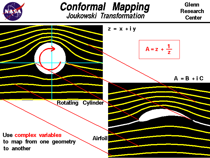
Joukowski transformation is a conformal mapping technique to derive an analytic solution of the flow around a Joukowski airfoil. First, consider the concept as indicated in the Figure below. The transformation maps the flow around a cylinder in cross flow (in the Z plane) onto the A plane where the circle is mapped to a Joukowski airfoil. This new curve preserves the conformal properties of the original circle, which means that it preserves angles (relevant to stream function and velocity potential) locally. As indicated by the lines, the following is mapped:

The cylinder surface $\rightarrow$ the Joukowski airfoil surface
The foremost stagnation point on the cylinder $\rightarrow$ the airfoil stagnation point near the leading edge.
The aft stagnation point on the cylinder $\rightarrow$ the airfoil trailing edge (Kutta Condition).
The flow is preserved in this mapping

Hence, at its basis, a Joukowsi airfoil is an airfoil created from “transforming” a cylinder (and its flow) to an airfoil using a special transformation.

Figure: Example of the conformal mapping through the Joukowski transform. The plots indicate the analytic solution of a rotating cylinder in cross flow to the transformation of the flow over a Joukowski airfoil.

Let’s now move to the details of the method. First, you must consider the Z-plane, which is a complex plane where the y-axis is imaginary and the x-axis is real. In the context of the complex potential function in the Z-plane, we can define $F(z)$ as

(37) $\begin{equation*} F(z)=\phi+i\psi. \end{equation*}$

Here, $\phi$ and $\psi$ need to be defined for the flow over a rotating cylinder which is the composition of a uniform flow + doublet + line vortex and is described here. Let’s walk through this in steps.

Starting with a free stream velocity we have a $phi$ and $psi$ . These are given as

(38) $\begin{equation*} \phi_{FS}=U_\infty x \end{equation*}$

Similarly, $\psi$ is given as

(39) $\begin{equation*} \psi_{FS}=U_\infty y \end{equation*}$

Constructing into the complex potential is as follows:

(40) $\begin{equation*} F_{FS}(z)=\phi_{FS}+i\psi_{FS}=U_\infty x + i U_\infty y \end{equation*}$

Recall that $z=x+iy$ , hence,

(41) $\begin{equation*} F_{FS}(z)=U_\infty z \end{equation*}$

This is a very simple flow and can be expanded to a flow with an angle of attack ( $\alpha$ ) with a free-stream velocity $\bar{V}=u_\infty\bar{i}+v_\infty\bar{j}=U_\infty\left(cos(\alpha)\bar{i}+sin(\alpha)\bar{j}\right)$ as

(42) $\begin{equation*} F_{FS}(z)=U_\infty e^{-i\alpha}z \end{equation*}$

Let’s now add the doublet and the line vortex (both at the origin, no angle of attack).

(43) $\begin{equation*} F(z)=U_\infty z+\frac{U_\infty R^2}{z} - i\frac{\Gamma}{2\pi}log(z) \end{equation*}$

Note that the 2nd and 3rd terms on the right-hand side are the doublet and line vortex, respectively. The differential of this gives us velocity, that is, $W(z)=F'=\frac{dF}{dz}=u-iw$ , which yields what looks like a normal differential as

(44) $\begin{equation*} W(z)=U_\infty -\frac{U_\infty R^2}{z^2} - i\frac{\Gamma}{2\pi}\frac{1}{z} \end{equation*}$

yielding the velocity field.

Examples: Complex potential flow over a rotating cylinder

Try this example matlab code. But sure to use the auto text cleanup.

clear

Uinf=1; %Free stream velocity

R=1; %Cyl radius

Gamma=10;%Ciruclation

%create mesh

x = meshgrid(-5:.1:5);

y = x’;

%create z on imaginary

z = x + i*y;

%clean up inside of cyl (basically let’s focus on only the flow)

for ii = 1:length(x)

for jj = 1:length(y)

if abs(z(ii,jj)) <= R

z(ii,jj) = NaN;

end

%create our complex potential function F

%%%%%Note, don’t forget to use term-by-term operations on z (use .* and ./)

F = Uinf*(z) + Uinf*R^2./z – i*Gamma/(2*3.14)*log(z);

%create our W

%%%%%Note, don’t forget to use term-by-term operations on z (use .* and ./ and .^2)

W = Uinf – Uinf*R^2./z.^2 + i*Gamma/(2*3.14)./z;

%plot

figure(1)

subplot(2,2,1)

contourf(x,y,real(F))

%xlabel(‘x (m)’)

ylabel(‘y (m)’)

title(‘Velocity Potential (phi)’)

set(gca,’Fontsize’,18)

subplot(2,2,2)

contourf(x,y,imag(F))

%xlabel(‘x (m)’)

ylabel(‘y (m)’)

title(‘Stream Function (psi)’)

set(gca,’Fontsize’,18)

subplot(2,2,3)

contourf(x,y,real(W))

xlabel(‘x (m)’)

ylabel(‘y (m)’)

title(‘u (m/s)’)

set(gca,’Fontsize’,18)

subplot(2,2,4)

contourf(x,y,-imag(W))

xlabel(‘x (m)’)

ylabel(‘y (m)’)

title(‘v (m/s)’)

set(gca,’Fontsize’,18)

figure(2)

contourf(x,y,sqrt(real(W).^2+imag(W).^2).^.5)

xlabel(‘x (m)’)

ylabel(‘y (m)’)

title(‘vmag (m/s)’)

set(gca,’Fontsize’,18)

Next, consider shifting the doublet and the line vortex from the origin, by some distance $mu$ . Note that $\mu=\delta x + i\delta y$ . We will also recover an angle of attack. The complex potential becomes

(45) $\begin{equation*} F(z)=U-\infty e^{-i\alpha} (z-\mu) +\frac{U_\infty R^2}{z-\mu} - i\frac{\Gamma}{2\pi}log(z-\mu) e^{i\alpha} \end{equation*}$

Note you can simply subtract $\mu$ from z. Similar to before, we obtain this differential

(46) $\begin{equation*} W(z)=U_\infty e^{-i\alpha}-\frac{U_\infty R^2}{(z-\mu)^2} + i\frac{\Gamma}{2\pi}\frac{1}{z-\mu}e^{i\alpha} \end{equation*}$

yielding the velocity field. See the example Matlab code below.

Examples: Lifting cylinder in flow with incidence and offset

clear
Uinf=1; %Free stream velocity
R=1; %Cyl radius
Gamma= 0.25*4*3.14*R*Uinf;%Ciruclation
aoa=25*pi/180; %aoa in rad
mu=0.5 +0.5*i;
%create mesh
x = meshgrid(-5:.1:5);
y = transpose(x);
%create z on imaginary
z = x + i*y;
%clean up inside of cyl (basically lets focus on only the flow)
for ii = 1:length(x)
for jj = 1:length(y)
if abs(z(ii,jj)-mu) <= R
z(ii,jj) = NaN; %comment this and see the high speed if this is not done.
end
end
end
%create our complex potential function F
%%%%%Note, don’t forget to use term-by-term operations on z (use .* and ./)
F = Uinf*((z-mu))*exp(-i*aoa) + Uinf*R^2./(z-mu) – i*Gamma/(2*3.14)*log((z-mu))*exp(i*aoa);
%create our W
%%%%%Note, don’t forget to use term-by-term operations on z (use .* and ./ and .^2)
W = Uinf*exp(-i*aoa) – Uinf*R^2./(z-mu).^2 + i*Gamma/(2*3.14)./(z-mu)*exp(-i*aoa);
%plot
figure(1)
subplot(2,2,1)
contourf(x,y,real(F))
%xlabel('x (m)’)
ylabel('y (m)')
title('Velocity Potential (\phi)')
set(gca,'Fontsize',18)
subplot(2,2,2)
contourf(x,y,imag(F))
%xlabel('x (m)')
ylabel('y (m)')
title('Stream Function (\psi)')
set(gca,'Fontsize',18)
subplot(2,2,3)
contourf(x,y,real(W))
xlabel('x (m)')
ylabel('y (m)')
title('u (m/s)')
set(gca,'Fontsize',18)
subplot(2,2,4)
contourf(x,y,-imag(W))
xlabel('x (m)')
ylabel('y (m)')
title('v (m/s)')
set(gca,'Fontsize',18)
figure(2)
contourf(x,y,sqrt(real(W).^2+imag(W).^2).^.5)
xlabel('x (m)')
ylabel('y (m)')
title('vmag (m/s)')
set(gca,'Fontsize',18)

Now let’s consider the Joukowski transform. The idea here is to transform from the z-plane (where z=x+iy), to the $\eta$ -plane (where $\eta=x'+iy'$ ). The mapping is as follows:

(47) $\begin{equation*} \eta=z+frac{R-mu}{z} \end{equation*}$

Examples: Joukowski transform

Try changing the inpu variables (R and mu) and see how things change.

clear

R=1;

mu=-0.2+i*0.1;

%loop over various angles

angle = 0:.01:2*pi;

%define the circle in the z plane

z_circle = R*(cos(angle)+i*sin(angle)) + mu;

%define the Jooukowski airfoil in the w plane

eta_airfoil = z_circle+(R-mu)^2./z_circle;

%plot comparisons

plot(z_circle)

hold on

plot(eta_airfoil)

hold off

Now move to the actual method. The steps as as follows:

Identify the stagnation points in the flow over a cylinder.
Change $mu$ such that the aft stagnation point falls on the real axis (i.e., no imaginary component)

(48) $\begin{equation*} W(z)=U_\infty e^{-i\alpha}-frac{U_\infty R^2}{(z-\mu)^2} + i\frac{\Gamma}{2\pi}\frac{1}{z-\mu}e^{i\alpha} \end{equation*}$

5 Chapter 5: Theory of Airfoil Lift Aerodynamics

Background Theory and Concepts

Airfoil

Baseline Aerodynamic Scaling, Parameters, and Concepts

Kutta condition

Kutta-Joukowski Theorem:

Thin Airfoil Models of Aerodynamics

Wiessinger’s approximation

Numerical Thin-Airfoil Theory

Thin-airfoil theory (TAT)

The Joukowski Airfoil

Potential Flow Represented in Complex Theory

License

Share This Book