
3 Chapter 3: Potential Flow Theory
Potential flow refers to the movement of a fluid (such as water or air) that relies on assumptions that are consistent with no viscosity or turbulence. This type of flow is often used as an idealized model to describe the behavior of fluids in certain situations, such as in fluid dynamics and aerodynamics. There are incompressible and compressible forms of the model.
In potential flow, the fluid moves in streamlines, which are lines that are tangent to the velocity vector at any given point. The fluid’s velocity is determined by the gradient of the flow’s scalar potential, the flow is irrotational, and the fluid’s pressure is yielded from the Bernoulli equation.
A key concept of potential flow is the construction of a complex flow scenario created by combining different flow models. Some examples of these flow models include:
- Source and sink flow: This occurs when at a point (or line in 2D) fluid is injected (source) or ingested (sink) from the flow. The resulting fluid flow will respond. Note that in aerodynamics we often use a “source sheet,” which is a continuous distribution of these. As we will see in class, these are often used to drive models of body thickness.
- Doublet flow: This occurs when a source and sink are placed virtually near each other. If the source and sink are coincident, they cancel. However, when very near they create a path of streamlines that form another scenario that looks like a cylinder (2D) and sphere (3D).
- Vortex flow: This occurs when there is a spinning motion in the fluid, such as a tornado or a whirlpool without the viscous core. The fluid will flow in a circular pattern around the center of rotation.
- Uniform flow: This occurs when the fluid is flowing at a constant velocity in a straight line.
It’s important to note that this type of flow is an idealization and only holds in situations where there is no viscosity and no turbulence in the fluid, and it’s mostly used as a theoretical underpinning for aerodynamic models.
Potential Flow Model
Prior to developing the potential flow model, we must rework how to describe velocity vectors. Potential flow demands defining two scalar fields, the velocity potential function ( ) and the stream function (
 ).
).
Velocity potential, , is 2D and 3D concept, and is, conceptually, a scalar that directly relates to velocity through the gradient of . That is, velocity always moves in the direction of increasing . In this context we obtain the Cartesian form as
(1) 
Which can be described in vector form as  . A simple analogy for may be elevation on a topographic map representing a mountain or a hill. The elevation is a scalar. However, if you have a ball it will fall down the steepest path (i.e., the lowest elevation gradient, so the analogy is similar but not exact).
Alternatively, the Stream function, is valid only in 2D, so it only applies to 2D bodies such as airfoils, cylinders, etc. For , a constant value yields a streamline (or a line a particle follows with slopes consistent with the local velocity). We obtain through tangency constraints, or
(2) 
(3) 
Now with these definitions, we can move into direct correspondence with the conservation equations.
First, consider the conservation of mass and how to get to potential flow. In the limit of a steady incompressible flow, mass conservation is as follows:
(4) 
Via the definition of velocity potential,  , we can simply insert the definition and we get
(5) 
Where the Laplacian is defined as follows
(6) 
and conservation of mass in our potential flow model can be represented as
(7) 
This is known as a Laplace equation which has some of the simplest solutions for a partial differential equation.
(8) 
which is important for various flows of interest.
We then bring the Conservation of Momentum back into the context of our Potential Flow model as a scalar relation in the form of the Bernoulli Equation:
(9) 
Recall that in the context of potential flow, Bernoulli Equation can extend beyond streamlines. Hence, it develops a path to recover pressure if needed for pressure integration.
In the context of potential flow, any equation that satisfies Laplace’s equation is virtually a valid solution for a flow in the limit of potential flow assumptions. The remaining gap is relating this to complex physical scenarios that are relevant to aerodynamic objects of interest, i.e., airfoils, wings, fuselages, etc.
The other aspect of potential flow is the irrotational flow condition, which enables a similar methodology in the context of the stream function. Recall that Irrotational flow is established by the state that the curl is equal to  , or
, or
(10) 
In the context of a 2D flow, we can expand this to
(11) 
Focusing only on the  term and Incorportating the defintition of
  and
and  in terms of the stream function yields
(12) 
Hence, the irrotational condition (fundamental to potential flow) demands that the Laplacian of must also be satisfied.
Elementary flows
Elementary potential flows refer to irrotational, inviscid and incompressible fluid flows that can are generated using simple mathematical functions (or flow elements). Examples of elementary potential flows include uniform flow (free stream), source/sink flow, vortex, and doublet. These flows can be used to model the behavior of real-world flows in certain conditions and provide a useful foundation for more complex fluid dynamics analysis. A very nice summary of these is provided in these tables of elementary flows which you should all have on hand. It is important to note these can be written in Cartesian and polar coordinates. As we will find in class, polar is useful for many scenarios.

Superposition
A critical concept for the path to developing complex aerodynamic configurations involves the concept of superimposition of individual potential flow solutions that are simple (elementary or flow elements) to construct models of more complex scenarios. There is a similar analogy with Legos. Each building block has various shapes that individually appear as blocks, but when combined they can recreate more elaborate shapes. In potential flow, our “Lego” blocks are fundamental solutions for (1) free stream flow, (2) source/sink, and/or (3)line vortex (amongst others). We add either a few, or many of these, together to formulate complex models that satisfy the governing equations.
Learning Objectives: Visual description of potential flow
Examples: Superposition
Question: Why can we simply add these simple models together and not violate the governing equation?
If the solution of an individual elementary flow (free-stream, vortex, source) satisfies Laplace’s equation, the result must be zero. It is a trivial solution! Since 0+0=0, we can easily see why superposition works.
Let’s test this out by adding a sink with a vortex at the origin:
(13) 
To evaluate mass conservation (in terms of velocity potential for polar coordinates, Eq. 7):
(14) 
Which becomes
(15) 
Yielding
(16) 
Which works! This can be done for any of these functions. Try on your own for:
- A Free Stream
- A Free Stream + Vortex @ Origin
- A Free Stream + Vortex @ Origin+ Dipole (doublet) @ Origin
An example of this is given in potentialflow.com.
In the context of and it should be clear that the superposition principles apply (e.g., we simply add of various elementary flows). It is also important to note that superposition similarly applies to velocities. That is, the addition of and is equivalent to the addition of the corresponding velocity fields ( ). It is important to note that and are trivial scalar additions, while involves vector addition. To explore why consider an example. Let’s assume we have elements 1 and 2 with velocity and velocity potential values given as
(17) 
(18) 
We can obtain as
(19) 
Or (note that  , hence,
  )
)
(20) 
It should be observed that the mathematics of addition within the integrals (linking velocity to ) is virtually the same as working with addition in an integrand. Therefore, the addition of (and ) is virtually the same as adding the velocity from each respective elementary flow.
Key Takeaways
- Laplace’s equation of is the conservation of mass in the limit of incompressible flow
- Laplace’s equation of implies an irrotational flow
- Bernoulli equation is one path to understanding pressure (and ultimately integrated to obtain force)
- Superposition enables combining the elementary flows, to form more complex flows.
- Superposition can be obtained from combining , , or .
Potential Flow Construction
In order to understand potential flow models, let’s explore various parameters and how they related to altering velocity in a given flow field. For now, lets solely focus on a uniform flow and the addition of sources.
Impact of a Source
Consider a simple scenario: Free Stream + source at origin  . How does the velocity vector change at
  ?
?
As can be observed in the figure below, the “free stream” has a velocity ( ) and velocity potential (
 ) that can be added everywhere in space to that source velocity (
 ) and velocity potential (
 ). Note that the free-stream velocity, is independent of space (but
  ). For the source, they tend to be a function of
  from the origin of the source, or
  and
and  . For convenience, at
  ,
,  to enable simple first examples. If we focus on the resulting velocity vector, we obtain a total vector that is the resultant vector of the free-stream and source components (as indicated in the figure). Note that the addition of (and ) are scalar additions, hence, do not demand vector addition. What you should focus on is how the total vector can change as we vary the parameters. If we increase the speed,
  , the total vector leans more towards
  to the x-axis (and slowing down does the opposite). Alternatively, we can change the source strength, m, to also change this vector orientation. Lastly, although we are fixed in space here, it is important to note that r is also important to change this velocity vector. Let us dig into the relevant details more to better understand.
If you are not following the concept, maybe a first cut could include exploring this flow in the potential flow simulator.
Alternatively, let’s explore analytically. Note for this case, the radial velocity from the source adds a vertical (or  -direction) component. This simplifies the process.
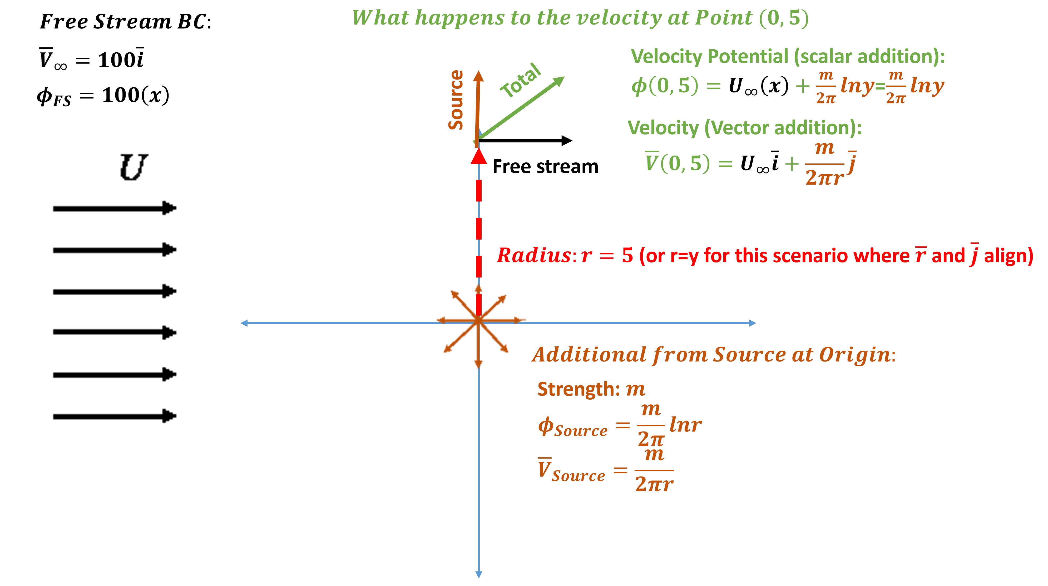
Velocity Potential: Velocity potential () is a scalar, and its addition is trivial. At we simply sum the velocity potentials at to obtain the combined value:
(21) 
To obtain velocity we could calculate:
(22) ![\begin{equation*} \overline{V}\left(0,5\right)=\left[\frac{\partial\phi}{\partial\ x}\overline{i}+\frac{\partial\phi}{\partial\ y}\overline{j}\right]_{@(0,5)}\ \end{equation*}](https://pressbooks.online.ucf.edu/app/uploads/quicklatex/quicklatex.com-64cc910a900db936a12c42cf4798cd8b_l3.png "Rendered by QuickLaTeX.com")
In general, it can be more complex because the source is defined radially, but here
(23) ![\begin{equation*} \overline{V}\left(0,5\right)=\left[U_\infty\overline{i}+\frac{m}{2\pi\ y}\ \overline{j}\right]_{@(0,5)} \end{equation*}](https://pressbooks.online.ucf.edu/app/uploads/quicklatex/quicklatex.com-14428eda2d2d1d6bfc0a9fea587951a9_l3.png "Rendered by QuickLaTeX.com")
As we will see, this is identical to adding velocity vectors.
Velocity Vector: Velocity vectors are also additive, and their addition is not too difficult, especially in this scenario. At we again sum the velocity vector contributions at to obtain the combined value. To obtain velocity we could calculate:
(24) 
However, this is complex because the source is defined radially. So the velocity vector becomes a function of m (which has units  ). For a source,
  , and the velocity points upward. Alternatively, for a sink m<0 and the velocity will point downward. As an example, if we want a vector to have a
  angle with respect to the x-axis, we need to match the
  and components, or:
(25) 
This is used to establish flow tangency with walls in a potential flow model.
Examples: Sample Matlab Script
Key Takeaways
In this simple example, we found that:
- The free stream acts like a free stream velocity in aerodynamics. It is a boundary condition.
- The source strength and distance control velocity vectors at specific points. This is important as it is used to specify “flow tangency” on surfaces.
Impact of Source Location
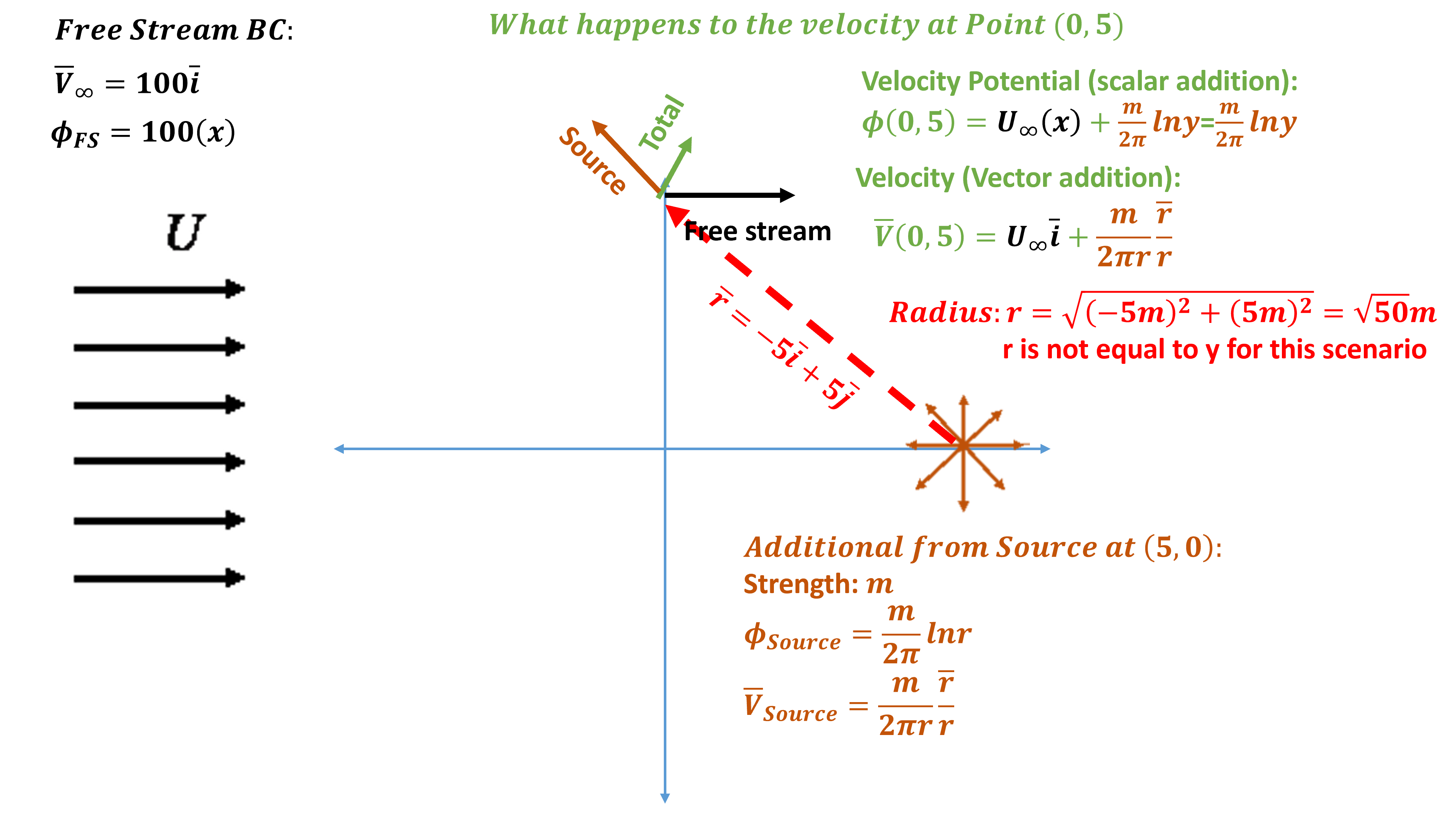
Consider a slightly more complex scenario: Free Stream + source at  . How does the velocity vector change at ?
You can try this in the potential flow simulator.
Alternatively, let’s explore analytically. For this case, the radial velocity from the source DOES NOT add a vertical (or -direction) component to the velocity vector. This can be seen in the vector addition in the figure above. This makes the process a little more complex. But let’s again explore using the velocity potential and vector addition.
Velocity Potential: Again, velocity potential () is a scalar, and its addition is trivial. At we simply sum the velocity potentials at to obtain the combined value:
(26) 
This scalar quantity is easy to work with but we have the same issue with obtaining velocity (mixing Cartesian and radial coordinates)
Velocity Vector: Velocity vectors are still additive, but demand to be accounted for in mixed coordinate systems. Similar to before, at we again sum the velocity vector contributions at to obtain the combined value. This time, however, the source acts in both the and directions. The magnitude is given by the radius
(27) 
The radial direction considered here demands decomposing into and components. This demands defining the vector as indicated in the figure. This vector provides direction in Cartesian coordinates. The direction is given by:
(28) 
Just a note, when we compute the velocity from a source at point  (which is in this example), we can generalize as follows:

We can now sum the velocity components of the free stream and source as follows:
(29) 
As an example, if we want a vector to have a  deg angle with respect to the x-axis, we need to match the and components, or:
(30) 
The result yields  . Hence, flow tangency with walls in a potential flow model can be constructed from sources in more complex configurations.
Examples: Matlab Script of uniform flow and source @ (5,0)
Key Takeaways
- A source induces a velocity in the radial direction which must be considered from the velocity “induced” by the source.
Multiple Sources
Consider a more complex scenario: Free Stream + source at + source at . How does the velocity vector change at ? The scenario is indicated in the Figure below and can be replicated in the potential flow simulator.

Again, we need to explore this scenario analytically. For this case, we need to add components from multiple sources. This can be seen in the vector addition in the figure above. This process is leading to how a panel code works. Lets us again explore using the velocity potential and vector addition.
Velocity Potential: Again, velocity potential () is a scalar, and its addition is trivial. At we simply sum the velocity potentials at to obtain the combined value:
(31) 
We continue to see the ease of working with this scalar quantity. But we also need to work with velocities.
Velocity Vector: Velocity vectors remain additive and this time include mixed coordinate systems and multiple sources. Similar to before, at we again sum the velocity vector contributions at to obtain the combined value. This time, however, two sources acts and need to be additively evaluated. When we sum the velocity components of the free stream and two source flows, we obtain:
(32) 
which becomes
(33) 
This can be expanded into a matrix multiplication as follows:
(34) 
Where  is a vector of influence coefficients, given as:
(35) ![\begin{equation*} {\overline{A}}^T=\frac{1}{2\pi}\left[\begin{matrix}\frac{\overline{r_1}}{\left|r_1\right|^2}&\frac{\overline{r_2}}{\left|r_2\right|^2}\\\end{matrix}\right] \end{equation*}](https://pressbooks.online.ucf.edu/app/uploads/quicklatex/quicklatex.com-4bcc0dfb22d76dd44f46667008170e4c_l3.png "Rendered by QuickLaTeX.com")
There is a vector of source strengths given as:
(36) ![\begin{equation*} \overline{m}=\left[\begin{matrix}m_1\\m_2\\\end{matrix}\right] \end{equation*}](https://pressbooks.online.ucf.edu/app/uploads/quicklatex/quicklatex.com-034eeb142e62cda14450ef762108b23e_l3.png "Rendered by QuickLaTeX.com")
This can be generalized to the following form where there are N_{sources}:
(37) 
The previous examples indicated how to find a source strength to specify a velocity direction. In this case, we have 1 equation and 2 unknowns ( and
and  ), hence, it is not solvable unless we fix one of the
  . Because of this we need to add a new equation to specify a velocity at another point. Here is a sample matlab/octave script:
Examples Matlabe script for multiple sources
Key Takeaways
- Multiple sources induce additive velocity, each with their own radial direction.
- Closing out the source strengths demands 1 equation for each source. This implies you will need to enforce velocity at two locations to obtain two sources.
Constructing a “no penetration” or “flow tangency” condition
Consider a more complex scenario: Free Stream + source at (0,5) + source at (5,0) and flat plate walls angled of +45 degrees (0,0) and -45 deg (5,5). The scenario is depicted in the figure below. Although the concept is complex, the underlying mathematics is not overly onerous.
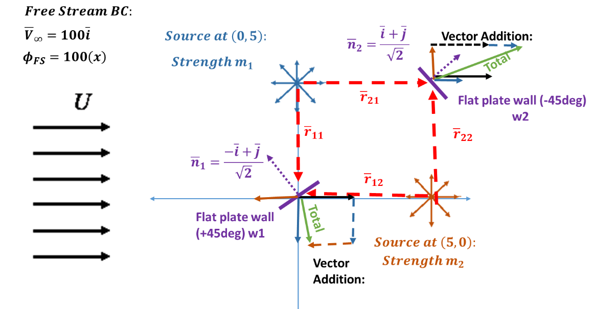
Now lets move into an approach to find source strengths. Recall from last time, we had two unknowns (m1 and m2) and one equation (velocity at (0,5)). This time, we have two flow tangency conditions giving us two equations (to close out the two unknowns). This time let’s just focus on the velocity vectors. Evaluating on wall 1 (w1) we get:
(38) 
which yields
(39) 
Note the convention,  is the radius from a source at location acting at point (or wall location) . This equation has two unknowns, and . At
  we seek to find flow tangency, that is flow is parallel to the wall. This is invoked in the condition where:
(40) 
Expanding this we obtain:
(41) 
Or
(42) 
Performing the same procedure on w2, we obtain:
(43) 
At this point, we have two equations and 2 unknowns, hence a solvable (and linear) system is formed. For this smaller case, a manual solution is possible. However, what we really seek it to extend to more complex and larger systems. Hence, we introduce a matrix form. We can combine the proceeding two equations into matrix in terms of ![\left[A\right]\overline{x}=\overline{b}](https://pressbooks.online.ucf.edu/app/uploads/quicklatex/quicklatex.com-fcaf9d957c560726a6c150d565bdcdad_l3.png "Rendered by QuickLaTeX.com") given as
given as
(44) ![\begin{equation*} \left[A\right]=\frac{1}{2\pi}\begin{bmatrix} \frac{\bar{r}_{11}\cdot\bar{n}_{1}}{\left|\bar{r}_{11}^2 \right|} & \frac{\bar{r}_{12}\cdot\bar{n}_{1}}{\left|\bar{r}_{12}^2 \right|} \\ \frac{\bar{r}_{21}\cdot\bar{n}_{2}}{\left|\bar{r}_{21}^2 \right|} & \frac{\bar{r}_{22}\cdot\bar{n}_{2}}{\left|\bar{r}_{22}^2 \right|} \end{bmatrix}. \end{equation*}](https://pressbooks.online.ucf.edu/app/uploads/quicklatex/quicklatex.com-3e89bc83839210bfd3b0b387112cb9b4_l3.png "Rendered by QuickLaTeX.com")
Here the elements of ![\left[A\right]](https://pressbooks.online.ucf.edu/app/uploads/quicklatex/quicklatex.com-1c0e0dcc393d2ca3499db29a2806b8e2_l3.png "Rendered by QuickLaTeX.com") are called influence coeffs and given as
are called influence coeffs and given as
(45) 
where the elements are given as  and
and
(46) ![\begin{equation*} \bar{b}=-\left[\begin{matrix}{\bar{V}}_\infty\cdot{\overline{n}}_1\\{\bar{V}}_\infty\cdot{\overline{n}}_2\\\end{matrix}\right] \end{equation*}](https://pressbooks.online.ucf.edu/app/uploads/quicklatex/quicklatex.com-84ee677cfb9d9de8ddd2cef7a1ce192e_l3.png "Rendered by QuickLaTeX.com")
where the elements are given as  . It is important that you see how this system is formed. Please review and make sure you understand it.
We can now solve using linear algebra techniques. Fortunately, we do not need fancy ones, and a brute force, matrix inversion, will do the trick. That is
(47) ![\begin{equation*} \overline{x}=\left[A\right]^{-1}\overline{b} \end{equation*}](https://pressbooks.online.ucf.edu/app/uploads/quicklatex/quicklatex.com-15813b6248c09307c85438a2a1da9ab1_l3.png "Rendered by QuickLaTeX.com")
In this solution,  is a vector of source strengths that will simultaneously satisfy flow tangency at the two constraints.
Examples: Sample matlab code to determine source strength to satisfy flow tangency
Key Takeaways
- For a series of unknown sources intended to drive flow tangency conditions. We need to satisfy flow tangency at one point for every source.
- The resulting equation set provides a linear system of equations specific to the flow tangency condition.
Source Panels
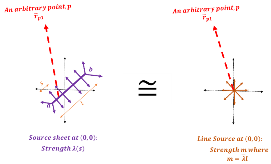
We can extend these concepts to what is referred to as a source panel. The concepts actually arrive from a basic potential flow concept of a source sheet shown in the diagram below:

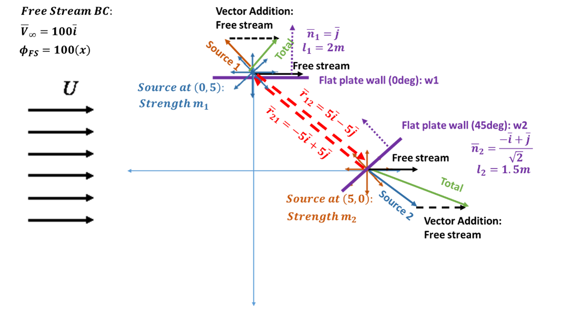
What we seek to do is position a “source sheet” on the walls of an aerodynamic body where we also seek to satisfy flow tangency (when also exposed to a free-stream velocity). We also want to simplify and treat the sheet as linear (i.e., line with slope and no curvature). To get to this scenario, consider: Free Stream + 2 m source sheet at (0,5) and positioned at a 0 deg orientation with a width of  . Then another source at (5,0) and angled at -45 deg (also 1.5m in width). Note that the source sheets are aligned with thin plates. The scenario is depicted below:
In this scenario (depicted below) we need to add two concepts:
- Accounting for sheets rather than point sources
- Accounting for self-influence (ie, the effect of the source sheet on itself)
To move from a source sheet to a point (or line) source we need to rework our source description. With the sheet we have an integral as follows:
(48) 
Note that the radius,  , and source/unit length, \lambda, are both a function of the sheet. The goal is to use a first-order method that uses a mean value of
  ,
,  , evaluated and the center of the source sheet (implying
  ). These assumptions enable the following simplification.
(49) 
Such an approximation is provided pictorially below.
Using this approach, our velocity equation for an arbitrary point p becomes:
(50)
Again, invoking the flow tangency condition:
(51) 
We obtain the following flow tangency constraints for w1:
(52) 
and for w2:
(53) 
In this scenario, we have an issue with  and
and  . The issue is that they both approach zero, leading to a divide by zero. We invoke the
(54) 
Using this approximation of the induced flow on itself, we eliminate the numerical issue. We can combine the proceeding two equations into matrix in terms of ![\left[A\right]\bar{x}=\bar{b}](https://pressbooks.online.ucf.edu/app/uploads/quicklatex/quicklatex.com-cdb92daacdd1755437918049242e9e76_l3.png "Rendered by QuickLaTeX.com") given as
given as
(55) ![\begin{equation*} \left[A\right]=\frac{1}{2\pi}\begin{bmatrix} \pi & \frac{\bar{r}_{12}\cdot\bar{n}_{1}}{\left|\bar{r}_{12}^2 \right|}l_2 \\ \frac{\bar{r}_{21}\cdot\bar{n}_{2}}{\left|\bar{r}_{21}^2 \right|}l_1 & \pi \end{bmatrix}. \end{equation*}](https://pressbooks.online.ucf.edu/app/uploads/quicklatex/quicklatex.com-f5ba598645b51f032628fa43397cce7f_l3.png "Rendered by QuickLaTeX.com")
These influence coefficients are generalized as
(56) 
Our source strengths are defined as
(57) ![\begin{equation*} \bar{x}=\left[\begin{matrix}\lambda_{avg,1}\\\lambda_{avg,2}\\\end{matrix}\right] \end{equation*}](https://pressbooks.online.ucf.edu/app/uploads/quicklatex/quicklatex.com-6636783624f7807ba1df12703696179b_l3.png "Rendered by QuickLaTeX.com")
where the elements are given as  . Finally, the remaining vector does not change and stays as
(58) ![\begin{equation*} \bar{b}=-\left[\begin{matrix}{\bar{V}}_\infty\cdot{\bar{n}}_1\\{\bar{V}}_\infty\cdot{\bar{n}}_2\\\end{matrix}\right] \end{equation*}](https://pressbooks.online.ucf.edu/app/uploads/quicklatex/quicklatex.com-536fbab420cb354c0195a26080966e4b_l3.png "Rendered by QuickLaTeX.com")
where the elements are given as  . Similar to before, we can now solver using linear algebra techniques and solve
(59) ![\begin{equation*} $\bar{x}=\left[A\right]^{-1}\overline{b}$. \end{equation*}](https://pressbooks.online.ucf.edu/app/uploads/quicklatex/quicklatex.com-56a85b4a79cde1f509cdc06eec615bc2_l3.png "Rendered by QuickLaTeX.com")
Which yields the final values of the source strengths that satisfies flow tangency.
Key Takeaways
- We move from a line source to a source sheet of finite length. This source sheet will become our “panels” that we will later use to represent a surface. We use a mean source strength and radius leading to a 1st order approximation. Anderson presents a higher-order method, but it is not instructive to look at it as a higher order.
- We also have to deal with singularity associated with the self-induced flow. The approach to remove this was given. Generally speaking, such singularities challenge potential flow methods
Panel Code
The aforementioned discussion leads to aerodynamic potential flow codes or panel codes. These codes are used to determine velocities and pressure distributions on objects. Note that this is only one path of potential flow. As we will see, it also leads to the foundational theory of aerodynamics. Panel codes can be thought of (at least as a first level) as a series of sources, sinks, vortex points, and/or doublets being positioned along panels that approximately (and discretely) represent an aerodynamic body. These panels can have various lengths and strengths.
There are also equations that can be formulated based on the summation of all the flow contributors (i.e., free stream velocity + induced flow from each panel) and the kinematic constraint of satisfying flow tangency on each panel. This forms a system of linear equations with unknowns that is solvable. This essentially extends the “source panels” section to closed bodies of interest. In this discussion, we aim to develop how sources can be combined with a uniform flow to develop a panel code within a stepwise procedure.

Step 1: Define the BCs
The first step demands free stream flight conditions including the speed and angle of attack. We also have to define the shape or paneling of the object. An example of this is depicted in the Figure above. It is important to note that each panel will (by default) be exposed to the free-stream velocity vector. Our goal aims to find the solution that yields flow tangency on each of the panels.
Step 2: Compute the control points
With the paneled airfoil, we now need to compute the “control points” on each panel. This is a point where we can approximately apply the sources and flow tangency. At this level let’s just assume we only need to evaluate at this control point. The control point is given as the midpoint of the panel:
(60) 
Note that  is the control point (vector) of panel i and
  and
and  are the vertices of panel i. Note that the panels should be ordered in a consistent direction around the closed body of interest (either clockwise or counterclockwise). This is important to keep the panel number as described correctly. Once defined, we formulate a model that satisfies flow tangency on the control points. The key need is to define the induced velocity from the other panels which involves calculated distances and directions.
Step 3: Compute the panel length and slope or normal vector
Closing this out demands a few other criteria:
- Panel length: we solve for an average strength, but it needs to consider being applied to a finite-length source sheet.

- Panel Slope: Enables us to set up a flow tangency condition (we can also define the normal vector)
 Or, the (outward) normal vector given as
Step 4: Now compute the influence coefficients
This is an extension of the previously discussed equations (in a 2-panel system).
(61) ![\begin{equation*} \left[A\right]=\frac{1}{2\pi}\begin{bmatrix} \pi & \frac{\bar{r}_{12}\cdot\bar{n}_{1}}{\left|\bar{r}_{12}^2 \right|}l_2 \\ \frac{\bar{r}_{21}\cdot\bar{n}_{2}}{\left|\bar{r}_{21}^2 \right|}l_1 & \pi \end{bmatrix} \end{equation*}](https://pressbooks.online.ucf.edu/app/uploads/quicklatex/quicklatex.com-7769ef24bb3df1d2cdf962eac0e15dd6_l3.png "Rendered by QuickLaTeX.com")
where the elements (called influence coefficients) and given as
(62) ![\begin{equation*} A_{i,j}=\frac{\bar{r_{ij}}\cdot{\bar{n}}_i}{\left|r_{ij}\right|^2}\ \bar{x}=\left[\begin{matrix}m_1\\m_2\\\end{matrix}\right] \end{equation*}](https://pressbooks.online.ucf.edu/app/uploads/quicklatex/quicklatex.com-0f875030a0948dd421605714a801efb2_l3.png "Rendered by QuickLaTeX.com")
where the elements are given as and
(63) ![\begin{equation*} \bar{b}=-\left[\begin{matrix}{\overline{V}}_\infty\cdot{\overline{n}}_1\\{\bar{V}}_\infty\cdot{\bar{n}}_2\\\end{matrix}\right] \end{equation*}](https://pressbooks.online.ucf.edu/app/uploads/quicklatex/quicklatex.com-09bab6d5f918ef879b8b2caad2542997_l3.png "Rendered by QuickLaTeX.com")
where the elements are given as .
Step 5: Reconstruct velocity and pressure coefficient
This is a vector approach that demands creating a function. Then 
Examples: Panel Code Walkthrough