30.8 Quantum Numbers and Rules

OpenStax

Chapter 30 Atomic Physics

30.8 Quantum Numbers and Rules

Summary

Define quantum number.
Calculate angle of angular momentum vector with an axis.
Define spin quantum number.

Physical characteristics that are quantized—such as energy, charge, and angular momentum—are of such importance that names and symbols are given to them. The values of quantized entities are expressed in terms of quantum numbers, and the rules governing them are of the utmost importance in determining what nature is and does. This section covers some of the more important quantum numbers and rules—all of which apply in chemistry, material science, and far beyond the realm of atomic physics, where they were first discovered. Once again, we see how physics makes discoveries which enable other fields to grow.

The energy states of bound systems are quantized, because the particle wavelength can fit into the bounds of the system in only certain ways. This was elaborated for the hydrogen atom, for which the allowed energies are expressed as $\boldsymbol{E_n \propto 1/n^2}$ , where $\boldsymbol{n = 1, 2, 3, \cdots }$ . We define $\boldsymbol{n}$ to be the principal quantum number that labels the basic states of a system. The lowest-energy state has $\boldsymbol{n = 1}$ , the first excited state has
$\boldsymbol{n = 2}$ , and so on. Thus the allowed values for the principal quantum number are

$\boldsymbol{n = 1, 2, 3, \cdots}$

This is more than just a numbering scheme, since the energy of the system, such as the hydrogen atom, can be expressed as some function of $\boldsymbol{n}$ , as can other characteristics (such as the orbital radii of the hydrogen atom).

The fact that the magnitude of angular momentum is quantized was first recognized by Bohr in relation to the hydrogen atom; it is now known to be true in general. With the development of quantum mechanics, it was found that the magnitude of angular momentum $\boldsymbol{L}$ can have only the values

$\boldsymbol{L = \sqrt{l (l + 1)}}$ $\boldsymbol{\frac{h}{2 \pi}}$ $\;\;\;\; \boldsymbol{(l = 0, 1, 2, \cdots , n - 1)}$

where $\boldsymbol{l}$ is defined to be the angular momentum quantum number. The rule for $\boldsymbol{l}$ in atoms is given in the parentheses. Given $\boldsymbol{n}$ , the value of $\boldsymbol{l}$ can be any integer from zero up to $\boldsymbol{n - 1}$ . For example, if $\boldsymbol{n = 4}$ , then $\boldsymbol{l}$ can be 0, 1, 2, or 3.

Note that for $\boldsymbol{n = 1}$ , $\boldsymbol{l}$ can only be zero. This means that the ground-state angular momentum for hydrogen is actually zero, not $\boldsymbol{h/2 \pi}$ as Bohr proposed. The picture of circular orbits is not valid, because there would be angular momentum for any circular orbit. A more valid picture is the cloud of probability shown for the ground state of hydrogen in Chapter 30.6 Figure 3. The electron actually spends time in and near the nucleus. The reason the electron does not remain in the nucleus is related to Heisenberg’s uncertainty principle—the electron’s energy would have to be much too large to be confined to the small space of the nucleus. Now the first excited state of hydrogen has $\boldsymbol{n = 2}$ , so that $\boldsymbol{l}$ can be either 0 or 1, according to the rule in $\boldsymbol{L = \sqrt{l (l + 1)} \frac{h}{2 \pi}}$ . Similarly, for $\boldsymbol{n = 3}$ , $\boldsymbol{l}$ can be 0, 1, or 2. It is often most convenient to state the value of $\boldsymbol{l}$ , a simple integer, rather than calculating the value of $\boldsymbol{L}$ from $\boldsymbol{L = \sqrt{l(l+1)} \frac{h}{2 \pi}}$ . For example, for $\boldsymbol{l = 2}$ , we see that

$\boldsymbol{L = \sqrt{2 (2+1)}}$ $\boldsymbol{\frac{h}{2 \pi}}$ $\boldsymbol{= \sqrt{6}}$ $\boldsymbol{\frac{h}{2 \pi}}$ $\boldsymbol{= 0.390h = 2.58 \times 10^{-34} \;\textbf{J} \cdot \textbf{s}}$

It is much simpler to state $\boldsymbol{l = 2}$ .

As recognized in the Zeeman effect, the direction of angular momentum is quantized. We now know this is true in all circumstances. It is found that the component of angular momentum along one direction in space, usually called the $\boldsymbol{z}$ -axis, can have only certain values of $\boldsymbol{L_z}$ . The direction in space must be related to something physical, such as the direction of the magnetic field at that location. This is an aspect of relativity. Direction has no meaning if there is nothing that varies with direction, as does magnetic force. The allowed values of $\boldsymbol{L_z}$ are

$\boldsymbol{L_z = m_l}$ $\boldsymbol{\frac{h}{2 \pi}}$ $\;\;\;\boldsymbol{(m_l = -l, -l +1, \cdots , -1, 0, 1, \cdots l - 1,l)}$

where $\boldsymbol{L_z}$ is the $\boldsymbol{z}$ -component of the angular momentum and $\boldsymbol{m_l}$ is the angular momentum projection quantum number. The rule in parentheses for the values of $\boldsymbol{m_l}$ is that it can range from $\boldsymbol{-l}$ to $\boldsymbol{l}$ in steps of one. For example, if $\boldsymbol{l = 2}$ , then $\boldsymbol{m_l}$ can have the five values –2, –1, 0, 1, and 2. Each $\boldsymbol{m_l}$ corresponds to a different energy in the presence of a magnetic field, so that they are related to the splitting of spectral lines into discrete parts, as discussed in the preceding section. If the $\boldsymbol{z}$ -component of angular momentum can have only certain values, then the angular momentum can have only certain directions, as illustrated in Figure 1.

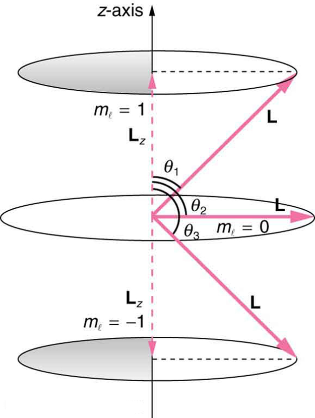
The image shows two possible values of component of a given angular momentum along z-axis. One circular orbit above the original circular orbit is shown for m sub l value of plus one. Another circular orbit below the original circular orbit is shown for m sub l value of minus one. The angular momentum vector for the top circular orbit makes an angle of theta sub one with the vertical axis. The horizontal angular momentum vector at original circular orbit makes an angle of theta sub two with the vertical axis. The angular momentum vector for the bottom circular orbit makes an angle of theta sub three with the vertical axis.

Example 1: What Are the Allowed Directions?

Calculate the angles that the angular momentum vector $\boldsymbol{L}$ can make with the $\boldsymbol{z}$ -axis for $\boldsymbol{l = 1}$ , as illustrated in Figure 1.

Strategy

Figure 1 represents the vectors $\boldsymbol{L}$ and $\boldsymbol{L_z}$ as usual, with arrows proportional to their magnitudes and pointing in the correct directions. $\boldsymbol{L}$ and $\boldsymbol{L_z}$ form a right triangle, with $\boldsymbol{L}$ being the hypotenuse and $\boldsymbol{L_z}$ the adjacent side. This means that the ratio of $\boldsymbol{L_z}$ to $\boldsymbol{L}$ is the cosine of the angle of interest. We can find $\boldsymbol{L}$ and $\boldsymbol{L_z}$ using $\boldsymbol{L = \sqrt{l (l+1)}\frac{h}{2\pi}}$ .

Solution

We are given $\boldsymbol{l = 1}$ , so that $\boldsymbol{m_l}$ can be +1, 0, or −1. Thus $\boldsymbol{L}$ has the value given by $\boldsymbol{L = \sqrt{l (l+1)} \frac{h}{2 \pi}}$ .

$\boldsymbol{L =}$ $\boldsymbol{\frac{\sqrt{l (l+1)}h}{2 \pi}}$ $\boldsymbol{=}$ $\boldsymbol{\frac{\sqrt{2}h}{2 \pi}}$

$\boldsymbol{L_z}$ can have three values, given by $\boldsymbol{L_z = m_l \frac{h}{2 \pi}}$ .

$\boldsymbol{L_z = m_l}$ $\boldsymbol{\frac{h}{2 \pi}}$ $\boldsymbol{=}$ $\boldsymbol{ \{ }$ $\begin{array}{cccc} \boldsymbol{\frac{h}{2 \pi},} & \boldsymbol{m_l} & \boldsymbol{=} & \boldsymbol{+1} \\[1em] \boldsymbol{0,} & \boldsymbol{m_l} & \boldsymbol{=} & \boldsymbol{0} \\[1em] \boldsymbol{- \frac{h}{2 \pi},} & \boldsymbol{m_l} & \boldsymbol{=} & \boldsymbol{-1} \end{array}$

As can be seen in Figure 1, $\boldsymbol{\textbf{cos} \;\theta = \textbf{L}_z / \textbf{L}}$ and so for $\boldsymbol{m_l = +1}$ , we have

$\boldsymbol{\textbf{cos} \;\theta _1=}$ $\boldsymbol{\frac{L_Z}{L}}$ $\boldsymbol{=}$ $\boldsymbol{\frac{\frac{h}{2 \pi}}{\frac{2h}{2 \pi}}}$ $\boldsymbol{=}$ $\boldsymbol{\frac{1}{\sqrt{2}}}$ $\boldsymbol{= 0.707}$

Thus,

$\boldsymbol{\theta _1 = \textbf{cos}^{-1} 0.707 = 45.0 ^{\circ}}$ .

Similarly, for $\boldsymbol{m_l = 0}$ , we find $\boldsymbol{\textbf{cos} \theta _2 = 0}$ ; thus,

$\boldsymbol{\theta _2 = \textbf{cos}^{-1} 0 = 90.0 ^{\circ}}$ .

And for $\boldsymbol{m_l = -1}$ ,

$\boldsymbol{\textbf{cos} \theta _3 =}$ $\boldsymbol{\frac{L_Z}{L}}$ $\boldsymbol{=}$ $\boldsymbol{\frac{- \frac{h}{2 \pi}}{\frac{2h}{2 \pi}}}$ $\boldsymbol{=}$ $\boldsymbol{- \frac{1}{\sqrt{2}}}$ $\boldsymbol{= -0.707}$ ,

so that

$\boldsymbol{\theta _3 = \textbf{cos}^{-1} (-0.707) = 135.0^{\circ}}$ .

Discussion

The angles are consistent with the figure. Only the angle relative to the $\boldsymbol{z}$ -axis is quantized. $\boldsymbol{L}$ can point in any direction as long as it makes the proper angle with the $\boldsymbol{z}$ -axis. Thus the angular momentum vectors lie on cones as illustrated. This behavior is not observed on the large scale. To see how the correspondence principle holds here, consider that the smallest angle ( $\boldsymbol{\theta _1}$ in the example) is for the maximum value of $\boldsymbol{m_l = 0}$ , namely $\boldsymbol{m_l = l}$ . For that smallest angle,

$\boldsymbol{\textbf{cos} \theta =}$ $\frac{L_z}{L}$ $\boldsymbol{=}$ $\boldsymbol{\frac{l}{\sqrt{l (l+1)}}}$ ,

which approaches 1 as $\boldsymbol{l}$ becomes very large. If $\boldsymbol{\textbf{cos} \theta = 1}$ , then $\boldsymbol{\theta =0 ^{\circ}}$ . Furthermore, for large $\boldsymbol{l}$ , there are many values of $\boldsymbol{m_l}$ , so that all angles become possible as $\boldsymbol{l}$ gets very large.

Intrinsic Spin Angular Momentum Is Quantized in Magnitude and Direction

There are two more quantum numbers of immediate concern. Both were first discovered for electrons in conjunction with fine structure in atomic spectra. It is now well established that electrons and other fundamental particles have intrinsic spin, roughly analogous to a planet spinning on its axis. This spin is a fundamental characteristic of particles, and only one magnitude of intrinsic spin is allowed for a given type of particle. Intrinsic angular momentum is quantized independently of orbital angular momentum. Additionally, the direction of the spin is also quantized. It has been found that the magnitude of the intrinsic (internal) spin angular momentum, $\boldsymbol{S}$ , of an electron is given by

$\boldsymbol{S = \sqrt{s (s+1)}}$ $\boldsymbol{\frac{h}{2 \pi}}$ $\;\;\; \boldsymbol{(s= 1/2 \;\textbf{for electrons})}$ ,

where $\boldsymbol{s}$ is defined to be the spin quantum number. This is very similar to the quantization of $\boldsymbol{L}$ given in $\boldsymbol{L = \sqrt{l (l + 1)} \frac{h}{2 \pi}}$ , except that the only value allowed for $\boldsymbol{s}$ for electrons is 1/2.

The direction of intrinsic spin is quantized, just as is the direction of orbital angular momentum. The direction of spin angular momentum along one direction in space, again called the $\boldsymbol{z}$ -axis, can have only the values

$\boldsymbol{S_z = m_s}$ $\boldsymbol{\frac{h}{2 \pi}}$ $\;\;\; \boldsymbol{(}$ $\boldsymbol{m_s = -}$ $\boldsymbol{\frac{1}{2}}$ $\boldsymbol{,+}$ $\boldsymbol{\frac{1}{2}}$ $\boldsymbol{)}$

for electrons. $\boldsymbol{S_z}$ is the $\boldsymbol{z}$ -component of spin angular momentum and $\boldsymbol{m_s}$ is the spin projection quantum number. For electrons, $\boldsymbol{s}$ can only be 1/2, and $\boldsymbol{m_s}$ can be either +1/2 or –1/2. Spin projection $\boldsymbol{m_s = +1/2}$ is referred to as spin up, whereas $\boldsymbol{m_s = -1/2}$ \ is called spin down. These are illustrated in Chapter 30.7 Figure 5.

Intrinsic Spin

In later chapters, we will see that intrinsic spin is a characteristic of all subatomic particles. For some particles $\boldsymbol{s}$ is half-integral, whereas for others $\boldsymbol{s}$ is integral—there are crucial differences between half-integral spin particles and integral spin particles. Protons and neutrons, like electrons, have $\boldsymbol{s = 1/2}$ , whereas photons have $\boldsymbol{s = 1}$ , and other particles called pions have $\boldsymbol{s = 0}$ , and so on.

To summarize, the state of a system, such as the precise nature of an electron in an atom, is determined by its particular quantum numbers. These are expressed in the form n, l,ml,msn, l,ml,ms —see Table 1 For electrons in atoms, the principal quantum number can have the values $\boldsymbol{n=1, 2, 3, \cdots}$ . Once $\boldsymbol{n}$ is known, the values of the angular momentum quantum number are limited to $\boldsymbol{l = 1, 2, 3, \cdots , n - 1}$ . For a given value of $\boldsymbol{l}$ , the angular momentum projection quantum number can have only the values $\boldsymbol{m_l = -l,-l + 1, \cdots , -1, 0, 1, \cdots ,l - 1,l}$ . Electron spin is independent of $\boldsymbol{n}$ , $\boldsymbol{l}$ , and $\boldsymbol{m_l}$ , always having $\boldsymbol{s=1/2}$ . The spin projection quantum number can have two values, $\boldsymbol{m_s=1/2}$ or $\boldsymbol{-1/2}$ .

Name	Symbol	Allowed values
Principal quantum number	$\boldsymbol{n}$	$\boldsymbol{1, 2, 3, \cdots}$
Angular momentum	$\boldsymbol{l}$	$\boldsymbol{0, 1, 2, \cdots n- 1}$
Angular momentum projection	$\boldsymbol{m_l}$	$\boldsymbol{-l, -l + 1, \cdots , -1, 0, 1, \cdots ,l-1,l \; (\textbf{or} \; 0, \pm 1, \pm 2, \cdots , \pm l)}$
Spin¹	$\boldsymbol{s}$	$\boldsymbol{1/2 \; (\textbf{electrons})}$
Spin projection	$\boldsymbol{m_s}$	$\boldsymbol{-1/2, +1/2}$
Table 1: Atomic Quantum Numbers

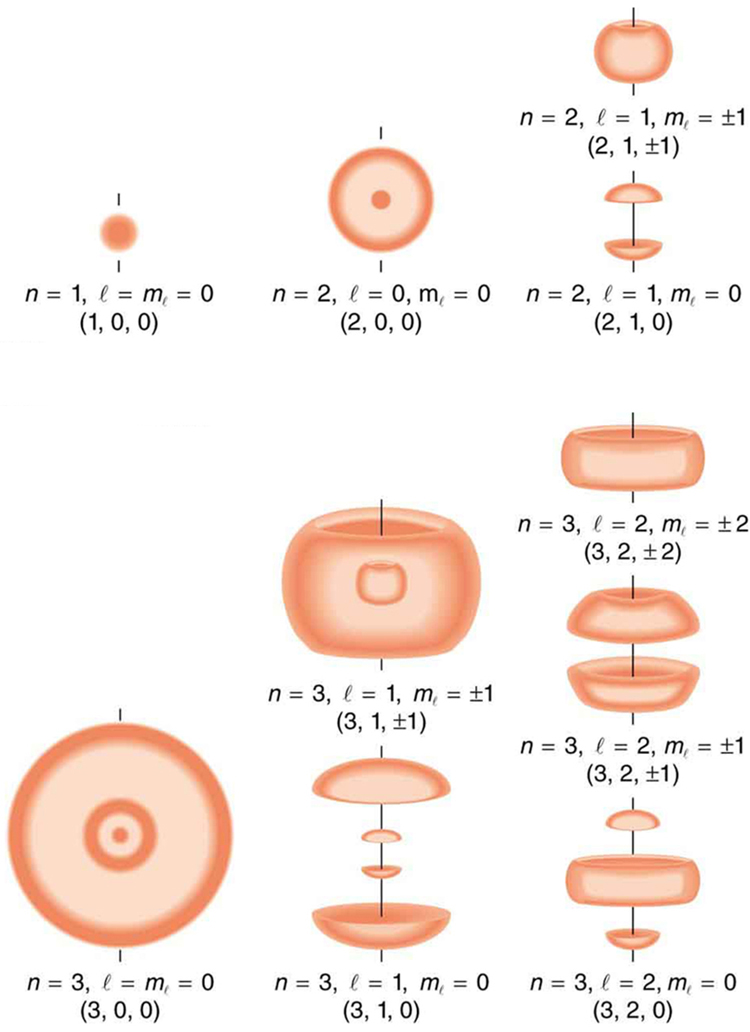
Figure 2 shows several hydrogen states corresponding to different sets of quantum numbers. Note that these clouds of probability are the locations of electrons as determined by making repeated measurements—each measurement finds the electron in a definite location, with a greater chance of finding the electron in some places rather than others. With repeated measurements, the pattern of probability shown in the figure emerges. The clouds of probability do not look like nor do they correspond to classical orbits. The uncertainty principle actually prevents us and nature from knowing how the electron gets from one place to another, and so an orbit really does not exist as such. Nature on a small scale is again much different from that on the large scale.

The image shows probability clouds for the electron in the ground state and several excited states of hydrogen. Sets of quantum numbers given as n l m subscript l are shown for each state. The ground state is zero zero zero. The probability of finding the electron is indicated by the shade of color.

We will see that the quantum numbers discussed in this section are valid for a broad range of particles and other systems, such as nuclei. Some quantum numbers, such as intrinsic spin, are related to fundamental classifications of subatomic particles, and they obey laws that will give us further insight into the substructure of matter and its interactions.

PhET Explorations: Stern-Gerlach Experiment

The classic Stern-Gerlach Experiment shows that atoms have a property called spin. Spin is a kind of intrinsic angular momentum, which has no classical counterpart. When the z-component of the spin is measured, one always gets one of two values: spin up or spin down.

Section Summary

Quantum numbers are used to express the allowed values of quantized entities. The principal quantum number $\boldsymbol{n}$ labels the basic states of a system and is given by
$\boldsymbol{n = 1, 2, 3, \cdots}$
The magnitude of angular momentum is given by
$\boldsymbol{L = \sqrt{l(l+1)}}$ $\boldsymbol{\frac{h}{2 \pi}}$ $\boldsymbol{(l=0, 1, 2, \cdots , n-1)}$

where $\boldsymbol{l}$ is the angular momentum quantum number. The direction of angular momentum is quantized, in that its component along an axis defined by a magnetic field, called the $\boldsymbol{z}$ -axis is given by

$\boldsymbol{L_z = m_l}$ $\boldsymbol{\frac{h}{2 \pi}}$ $\;\;\;\boldsymbol{(m_l = -l, -l+1, \cdots , 1, 0, 1, \cdots l-1,l)}$

where $\boldsymbol{L_z}$ is the $\boldsymbol{z}$ -component of the angular momentum and $\boldsymbol{m_l}$ is the angular momentum projection quantum number. Similarly, the electron’s intrinsic spin angular momentum $\boldsymbol{S}$ is given by

$\boldsymbol{S= \sqrt{s (s+1)}}$ $\boldsymbol{\frac{h}{2 \pi}}$ $\;\;\;\boldsymbol{(s = 1/2 \;\textbf{for electrons})}$

$\boldsymbol{s}$ is defined to be the spin quantum number. Finally, the direction of the electron’s spin along the $\boldsymbol{z}$ -axis is given by

$\boldsymbol{S_z = m_s}$ $\boldsymbol{\frac{h}{2 \pi}}$ $\boldsymbol{(}$ $\boldsymbol{m_s = -}$ $\boldsymbol{\frac{1}{2}}$ $\boldsymbol{,+}$ $\boldsymbol{\frac{1}{2}}$ $\boldsymbol{)}$ ,

where $\boldsymbol{S_z}$ is the $\boldsymbol{z}$ -component of spin angular momentum and $\boldsymbol{m_s}$ is the spin projection quantum number. Spin projection $\boldsymbol{m_s = +1/2}$ is referred to as spin up, whereas $\boldsymbol{m_s= -1/2}$ is called spin down. Table 1 summarizes the atomic quantum numbers and their allowed values.

Conceptual Questions

1: Define the quantum numbers $\boldsymbol{n}$ , $\boldsymbol{l}$ , $\boldsymbol{m_l}$ , $\boldsymbol{s}$ , $\boldsymbol{m_s}$ .

2: For a given value of $\boldsymbol{n}$ , what are the allowed values of $\boldsymbol{l}$ ?

3: For a given value of $\boldsymbol{l}$ , what are the allowed values of $\boldsymbol{m_l}$ ? What are the allowed values of $\boldsymbol{m_l}$ for a given value of $\boldsymbol{n}$ ? Give an example in each case.

4: List all the possible values of $\boldsymbol{s}$ and $\boldsymbol{m_s}$ for an electron. Are there particles for which these values are different? The same?

Problem Exercises

1: If an atom has an electron in the $\boldsymbol{n=5}$ state with $\boldsymbol{m_l=3}$ , what are the possible values of $\boldsymbol{l}$ ?

2: An atom has an electron with $\boldsymbol{m_l = 2}$ . What is the smallest value of $\boldsymbol{n}$ for this electron?

3: What are the possible values of $\boldsymbol{m_l}$ for an electron in the $\boldsymbol{n = 4}$ state?

4: What, if any, constraints does a value of $\boldsymbol{m_l=1}$ place on the other quantum numbers for an electron in an atom?

5: (a) Calculate the magnitude of the angular momentum for an $\boldsymbol{l = 1}$ electron. (b) Compare your answer to the value Bohr proposed for the n=1n=1 size 12{n=1} {} state.

6: (a) What is the magnitude of the angular momentum for an $\boldsymbol{l=1}$ electron? (b) Calculate the magnitude of the electron’s spin angular momentum. (c) What is the ratio of these angular momenta?

7: Repeat Chapter 30.8 Exercise 6 for $\boldsymbol{l=3}$ .

8: (a) How many angles can $\boldsymbol{L}$ make with the $\boldsymbol{z}$ -axis for an $\boldsymbol{l = 2}$ electron? (b) Calculate the value of the smallest angle.

9: What angles can the spin $\boldsymbol{S}$ of an electron make with the $\boldsymbol{z}$ -axis?

Footnotes

1 The spin quantum number s is usually not stated, since it is always 1/2 for electrons

Glossary

quantum numbers: the values of quantized entities, such as energy and angular momentum

angular momentum quantum number: a quantum number associated with the angular momentum of electrons

spin quantum number: the quantum number that parameterizes the intrinsic angular momentum (or spin angular momentum, or simply spin) of a given particle

spin projection quantum number: quantum number that can be used to calculate the intrinsic electron angular momentum along the $\boldsymbol{z}$ -axis