Main Body
Chapter 1, Measuring Matter and Motion
brueckner
 “…for all the difficulty of philosophy seems to consist in this—from the phaenomena of motions to investigate the forces of nature, and then from these forces to demonstrate the other phaenomena.”
—Sir Isaac Newton, preface to Principia
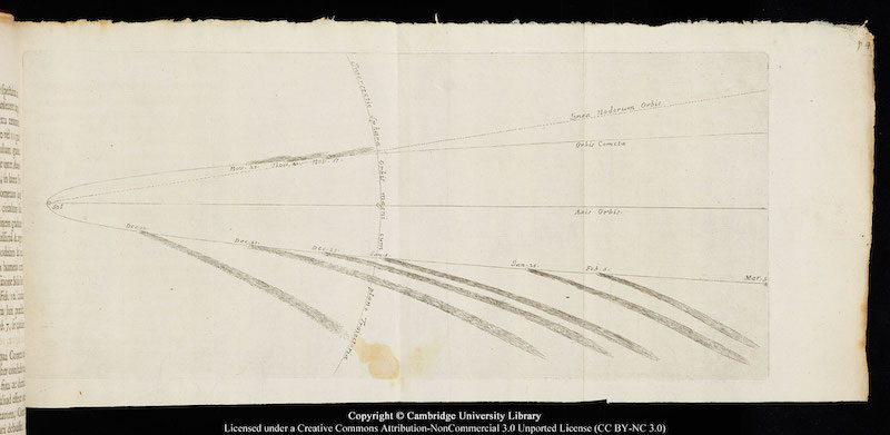
Sir Isaac Newton followed Galileo’s program by breaking down his subject into a few subcategories: motion in itself, then forces as the cause of changes to motion, and finally extending the understanding of forces to “other phenomena” like the orbit of a comet. And he did it all in a mathematical manner. In this chapter, we shall work out the first basic task:
- measuring matter and motion,
- defining positions,
- defining velocity and
- defining acceleration.
We will do so conceptually and mathematically, with a bias toward simplicity. And in simplicity, we will have a set of tools and building materials to construct understanding of more elaborate phenomena—comets, ocean waves, atoms, and any other physical systems.
1.1 How Does One Measure a Position in Three-Dimensional Space?
If you walk around in certain neighborhoods of a big city like New York or a small town like Clewiston, Florida, your journey might consist of lefts and rights, measurable distances after each turn, from your starting point, to your destination. To tell a fellow scientist where you are, you would write a message with a pair of numbers, for example, 2 blocks east, 3 blocks north from the starting point, to the destination point. If you were to offer your fellow scientist a map of your route, it would show a series of perpendicular, connected line segments; on a piece of graph paper, we traditionally call the perpendicular directions x and y. If your destination was a three-storey office building, with a coffee shop on the ground floor, an accountant’s office on the second floor and an architect’s office on the third floor, your message would include a third number: the number of the floor. Are you inviting your scientist friend to have a cup of coffee, double check your IRS tax forms, or look over the plans for building a new beach house?
In general, three numbers accurately and uniquely identify a spatial location, with each number specifying a certain distance from the starting point. So your spatial system must also include a well-identified starting point; traditionally, we give this special location the special set of three numbers (0, 0, 0). A mathematician would call it the origin. In addition to using three numbers per location and having one special origin, you would also need to specify what kind of distance measuring system your numbers use. That is, does (2, 3, 3) refer to 2 blocks east, 3 blocks north, and 3rd floor, where the architects work, or to 2 miles east, 3 miles east, and 3 miles up in the sky—where an airplane might be? Most of our distance measurements in this book will be meters or some derivative of the meter, like a kilometer, a nanometer, or an Angstrom.
Example 1
SCIENTIFIC NOTATION FOR METERS, NANOMETERS, AND ANGSTROMS
The meter is about half the size of a tall adult, and is good for many everyday measuring tasks, like measuring the size of a classroom. However, for measuring the size of an atom, the nanometer, abbreviated nm, is better.
- A nanometer is a billionth fraction of a meter, 0.000000001 meter: in scientific notation, one expresses it as 1 × 10⁻⁹ m, with the −9 signifying, of course, that the numeral 1 is nine places to the right of the decimal point. Meters to nanometers are 1:109, 1.0 nm = 1×10⁻⁹.
- An Angstrom, abbreviated Å, is even smaller, a ten-billionth of a meter, 1 × 10⁻¹⁰ m, as developed by Prof. Anders Ångström for the systematic study of the spectrum of colors in sunlight. Nanometers and Angstrom units are 1:10, 1.0 nm = 10 A.
When making calculations on your calculator, a regular scientific calculator or a cell phone calculator, it is important to handle its scientific notation carefully. On a written examination, you might write in a wavelength from a hydrogen atom as 6.56 = 10−7 m, for instance, and a grader could easily mark it “correct.” Pure hydrogen does emit light at this wavelength, the famous H-alpha spectral line. When using clickers during a lecture, however, it is sometimes convenient to type in a whole number for one’s answer—in this case, the instructor might direct you to type in your answer to the nearest nanometer. How does one get from 6.56 × 10⁻⁷ m to a whole number of nanometers? On a calculator, 6.56 × 10⁻⁷ looks like this:
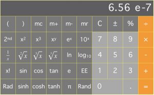
Divide that answer by 1 × 10⁻⁹, which is the conversion factor from meters to nanometers.
 ÷ 1 E ± 9 = 656
You use the same method you’d use if you had a box of 240 donuts and a policeman asked you, “Before I decide to arrest you, tell me, how many dozen donuts you have in that box?” As you slowly put down the box of donuts, you also mentally divide 240 by 12, to get the answer, “Twenty dozen, your honor.” The same idea helps you with wavelengths: divide by 1 × 10⁻⁹.
Similarly, if the clicker instruction called for the numeric part of an answer in Angstroms, you would divide by 1×10⁻¹⁰. That would give you an answer 6560 Å. All three are correct answers, 6.56 × 10⁻⁷ m, 656 nm and 6560 Å. You could even look it up: the wavelength of hydrogen’s H-alpha line on nasa.gov cites the hydrogen alpha wavelength, to four significant figures, as 656.3 nm and 6563 Å.
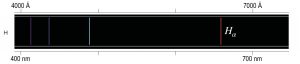
 . The other lines are H-beta (aqua), H-delta (purpley-blue), H-gamma (violet)
Occasionally, we will refer to miles, yards, feet, inches and other English units of measurement, simply because they are so familiar here in the USA. That is, everyone knows what it means to say, “Don’t give an inch!” But telling a friend that you escaped by a mere nanometer might not get the point across. Nonetheless, most of our work will be in meters.
1.2 What Is a Meter and How Was It Invented?
Scientists have set up many of our physical measures in reference to everyday events, like freezing water, which they use as a point on a temperature scale. For a meter, the everyday object is Earth itself, and the meter was initially set to be one ten-millionth of the distance from the Equator to the North Pole along the line of longitude that passes through Paris, France.
From that Earth-measuring result, scientists then constructed a flat, rigid bar made of an alloy of platinum and iridium metals, with the meter marked out between two lines on the bar. But Earth is not a perfect sphere; it is slightly flattened at the north and south poles. So, in 1960, a new standard object was used, the element krypton. It emits a specific orange light, for which the wavelength has been measured carefully: 1,650,763.73 waves of this color are one meter. In 1983, the final refinement to the meter was to set it as the distance light of any color travels in the time interval 1/299,792,458 of a second. This means that a physicist must be able to distinguish this fraction of a second from other fractions:
![\[\frac{1}{299792759}\text{ vs. }\frac{1}{299792758}\text{ vs. }\frac{1}{299792757}\]](https://pressbooks.online.ucf.edu/app/uploads/quicklatex/quicklatex.com-d555f2ed014b3215ab5fdca80332ec55_l3.png "Rendered by QuickLaTeX.com")
Using lasers, physicists are able to make these kinds of ultraprecise measurements now.
So the meter began its career as a fraction of a line of longitude running from the Equator to the North Pole, through Paris, and is now set using another fraction, a fraction of a second. This leads us to the next topic: time and time intervals.
1.3 What Is a Second and How Was It Invented?
The ancient Sumerian civilization of Mesopotamia used a numbering system based on 60. We see the remnants of this system in many places, like 60 seconds in one minute of time and 360 degrees in one full circle. Egyptians considered a single day to be divided into twelve hours of daylight and twelve hours of darkness, neglecting the seasonal variation of longer days in summer, shorter days in winter. In the modern era, we think of a single day as the time at high noon, when the sun is due south on a given day, to high noon on the next day. This measure is a solar day. An hour of that day, divided Sumerian style into 60 equal parts gives us a minute.
Each minute divided Sumerianly again, into 60 equal parts, gives us the second. But the Earth’s daily spin is slowing down slightly over the centuries, so the most modern method uses atoms and their electromagnetic radiation. This is the cesium atomic clock. All cesium atoms emit a frequency of microwave radiation slightly above the cell phone frequency 1.9 GHz, 1.9 billion cycles per sec. The useful frequency from cesium atoms is 9,192,631,770 Hz, or 9.192631770 GHz. We know this frequency to 10 significant figures! It means that this microwave’s electromagnetic field wiggles at the rate of 9,192,631,770 times per second. So the physicists in the laboratory count out 9,192,631,770 full wiggles and call that one second. Their electronics and software can handle that counting task.
This measurement is different than taking a fraction of the Earth’s circumference or a fraction of a solar day. It measures the duration of a large bundle, a specific number of electromagnetic waves from the cesium atom.
1.4 What Is a Kilogram, and How Was It Invented?
The kilogram is based on liquid water and the meter. Each kilogram contains one thousand grams, and one gram is defined as the mass of a cubic centimeter of liquid water at the melting point, 0°C.
(A cubic centimeter of volume, cm3, is also known as a milliliter, ml.) One thousand grams, a kilogram, is the mass of one liter of water, one thousand cubic centimeters, one thousand milliliters.
The kilogram is a mass. One way to measure an unknown mass is with a common measurement device, a balance.

“balance”by hans s is licensed under CC BY-ND 2.0![]()
![]()
![]()
Take an object for which you want to find the mass, in kilograms. Place the object in one side of the balance, then begin stacking liter bottles of water into the other side of the balance. When the two sides balance evenly, at the same height, neither side tilting downward, count the number of liters of water, and that will be the mass of the object, in kilograms.
1.5 Isn’t a Kilogram Actually a Weight, Not a Mass?
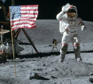
A kilogram is a mass, not a weight. Here is how you can distinguish between these two concepts. If you took your object to the moon, it would balance with the same number of liter bottles of water. However, your object would feel lighter on the moon, as you would, yourself. That is the difference: lighter weight on the moon, but same mass, same number of liter bottles in the balance. Just remember how high those Apollo astronauts could jump on the moon, even wearing their 28 kg space suit!
We will discuss weight in more detail in Chapter 3.
1.6 How Can We Make an Adequate Prediction of an Object’s Position at a Later Time?
The quantities we must use to predict the position of a baseball 3 seconds from now or a comet 300 years from now are these three quantities:
- the object’s position right now,
- the object’s velocity right now, and
- the rate at which the object’s velocity changes over time, that is, its acceleration.
The first two quantities, the object’s initial conditions, change over time according to the accelerations it might or might not experience. We have already described positioning, so let’s turn to motion itself, beginning with the idea of velocity.

1.7 How Does a Velocity Encode Where an Object Is Going and How Soon It Will Get There?
The idea of velocity is the coupling of direction and speed. If you are in a car, it is not enough simply to know the speed in miles per hour from the speedometer if you are trying to figure out where you are going:
- west to get donuts at Dunkin Donuts,
- south to the Waterford Lakes mall, or
- north to get groceries at Publix.
Your car has a steering wheel for a purpose. You must use the steering wheel carefully to aim your car in the right direction in your quest for donuts. This idea, “Where am I going?” requires you to specify a direction. It is therefore something you can express with an arrow, known mathematically as a vector.

In the figure above, the first view of the red car shows a relatively slow rate of motion, compared to the second view. The car’s first velocity arrow is shorter, the car’s second velocity arrow is longer. This brings us to discussion of speed.
In addition to the direction, a velocity must specify the speed, how quickly your vehicle is getting along toward its destination—how many miles for each minute of travel, how many miles per hour of travel, how many kilometers per hour of travel, how many meters per second of travel.
Let’s say that, in this view, rightward is west on University Boulevard. After taking a look at the speedometers, one might write down the following velocities,  and
and  :
:
![\[\vec{v}_1=5.0\frac{m}{s}\text{, west}\]](https://pressbooks.online.ucf.edu/app/uploads/quicklatex/quicklatex.com-818e52589d26d0d2428a80f77cc1ac29_l3.png "Rendered by QuickLaTeX.com")
![\[\vec{v}_2=8.0\frac{m}{s}\text{, west}\]](https://pressbooks.online.ucf.edu/app/uploads/quicklatex/quicklatex.com-8cd732e8390192cacca2d540c3a0acf0_l3.png "Rendered by QuickLaTeX.com")
(The tiny arrow over the symbol  means we are thinking of a vector quantity, with a direction, not just a simple, directionless number.) Heading for the mall at 20 m/s, you’d write a third velocity,
  . Every second of driving gets you another 20 meters closer to the mall.
1.8 How Does One Calculate the Exact Direction of Travel?
You can specify direction like a naval officer, who lays a course from Mayport, Florida, to Portsmouth, England, bearing 45° from true north. In layman’s terms, that is northeast relative to Jacksonville. When working out a complex set of directions, trigonometry is required. In this course, however, we will not work trigonometric calculations for angles. For us, a normal compass rose of eight directions,

- North (N)
- Northeast (NE), 45° clockwise from North
- East (E)
- Southeast (SE), 45° clockwise from East
- South (S)
- Southwest (SW), 45° clockwise from South
- West (W)
- Northwest (NW), 45° clockwise from West.
will be sufficient. For instance, if you climb to an upper floor of the John C. Hitt Library and look out the windows across the reflecting pond and slightly to the right, you’ll see the Teaching Academy. Depending on the window you use, the direction is about 245° clockwise from true north, but it is acceptable for us to say its direction is southwest.
1.9 How Does One Calculate Speed of Travel?
The customary speed rating system in the United States is mph, miles per hour. This gives us a clue about the basic calculation method: it is a distance interval divided by a time interval. If you make a distance of 7.8 miles in 2.0 hours, your speed is
![\[v=\frac{7.8\:miles}{2.0\:hours}=3.9\:mph\]](https://pressbooks.online.ucf.edu/app/uploads/quicklatex/quicklatex.com-12871e434ed26f1e6aad7648f41b5ba6_l3.png "Rendered by QuickLaTeX.com")
Converting that to meters per second, that speed is v = 1.74 m/s.
Example 2
Let’s work out the conversion of mph to m/s, and from m/s to mph.


So 
Similarly, 
I always remember the second conversion, so that I can translate a metric system speed in m/s to something I intuitively savvy, mph. So I see a speed like 4 m/s and I mentally estimate  which is about 8.8 or maybe 9 mph, a slow speed for a car or a fast speed for a runner. If that is not “close enough for government work,” I look it up in the book and multiply carefully on my calculator: 8.936 mph.
The generic formula for speed is
![\[v=\frac{\text{displacement}}{\text{elapsed time}}\]](https://pressbooks.online.ucf.edu/app/uploads/quicklatex/quicklatex.com-b4fc37c586cc7f6e33a088a0bac03155_l3.png "Rendered by QuickLaTeX.com")
If you measure a distance interval along the x-axis, from position x1 at time t1 to position x2 at time t2, we can use a compact formula for the speed, viz.
Definition of displacement Δx: 
Definition of elapsed time Δt: 
Formula for speed: 
This notation, using the symbol  , denotes a difference, a subtraction of two values, and it is usually the earlier value, for example, x1, subtracted from the later value, x2.
So if your time and position measurements out on the Florida Turnpike are the following,
| Event | Position | Time |
| 1 | Mile marker 259 | 1:55:08 PM, 9/31/15 |
| 2 | Mile marker 266.8 | 3:55:08 PM, 9/31/15 |
then the numerator of the formula is
![\[\Delta x = \left(266.8\:miles-259.0\:miles\right)=7.8\:miles\]](https://pressbooks.online.ucf.edu/app/uploads/quicklatex/quicklatex.com-2ca328cf286a695a7fed522ea7404c46_l3.png "Rendered by QuickLaTeX.com")
and the denominator elapsed time is
![\[\Delta t=\left(3:55:08 - 1:55:08\right)=2.00\:hour\]](https://pressbooks.online.ucf.edu/app/uploads/quicklatex/quicklatex.com-399cb2bc927e39e155abe724f4c03af6_l3.png "Rendered by QuickLaTeX.com")
resulting in speed  .
.
1.10 What Is the Difference Between an Average Speed and an Instantaneous Speed?
What if you took a 30-minute nap and donuts break along the way at the Turkey Lake Service Plaza, at mile marker 263? How does that affect your speed calculation? It does not affect the above calculation, as long as you call it an average speed. An average adds up a number of measurements and then divides by how many measurements you have. If you took a note of the speed every minute, then there would be 120 numbers to average. If you take a nap, some of those minute-by-minute speed numbers will be zeroes. Others will necessarily be higher than 3.9 mph. A few will be larger than zero but less than 3.9 mph. The speed formula only tells you the average speed for the time interval in question, 1:55–3:55 PM. It cannot tell you the speed at any specific instant of time—your instantaneous speed. Even the minute-by-minute speeds from the speedometer or GPS device are average speeds for very small elapsed time intervals built into the car’s speedometer system or the GPS device. However, the speedometer reading is still a pretty good way to think about the instantaneous speed of an object.
Another way to distinguish between average and instantaneous speed, average and instantaneous velocities, is to think about our task, describing and predicting the state of motion of a physical object. An average speed is useful, but it might not describe your actual speed at some instant of time. It gives an imperfect, approximate description of the state of motion. The instantaneous speed purports to describe the exact speed at some specific instant of time, like an average speed for an infinitesimally small time interval. This would be a perfect description of the state of motion. Somewhere in between average and instantaneous is the informal speedometer speed, fairly close to the instantaneous speed, but actually an average speed over a finite, short time interval.
| Δx | Δt | Knowledge of the state of motion | |
| Average speed | Any size | Any size | Approximate |
| “Speedometer speed” | Any size | Very small, less than 1.00 second | Decent |
| Instantaneous speed | Any size | Infinitesimally small | Theoretically exact, so a perfect description |
1.11 The Tortoise and the Hare Race for Donuts

Now think of this in terms of the fable of the tortoise and the hare. The hare is capable of much higher instantaneous speeds than the tortoise can even think about.
But, in the fable, the hare takes naps and lowers his average speed so much that he gets dusted by the tortoise. And the tortoise’s instantaneous speeds at any time are very close to his average speed because, in the fable, he just cooks along at maybe 100 feet per minute, but he does so without variation, never wavering, and wins the prize.
Here are the tables of average speeds for the tortoise and hare, for a hypothetical race from the studying at the library to Dunkin Donuts.
The tortoise gets up to speed in his first minute, from zero to 100 feet per minute, so his average speed for that first minute is 50 ft/min. Then he chugs along at 100 ft/min for the rest of the thirty minutes he needs to get to Dunkin Donuts.

The hare is erratic. He jams out at high speed, with average speed of 860 ft/min in that first minute. So at the end of that first minute, he is 860 feet from the library. In the next minute, his average speed is down to 464 ft/min, covering another 464 feet of travel in that second minute, reaching a total distance from the library of 1324 feet.
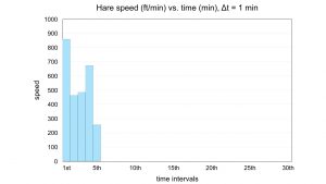
He speeds up slightly in the third minute, puts on another burst of speed in the fourth minute. The hare eases down to 257 ft/min in the fifth minute: Dunkin Donuts is in sight, and his total distance is 2741 feet. He looks back, and the tortoise, only 450 feet from the library, is so far back he cannot be seen. So Mr. Smart Guy, the hare, settles down for a quick nap. “No problem,” he says to himself, “I got this.”
Not really.
|
Time (minutes) |
Tortoise speed (ft/min) |
Hare speed (ft/min) |
|
1 |
50 |
860 |
|
2 |
100 |
464 |
|
3 |
100 |
485 |
|
4 |
100 |
675 |
|
5 |
100 |
257 |
|
6 |
100 |
0 |
|
7 |
100 |
0 |
|
8 |
100 |
0 |
|
9 |
100 |
0 |
|
10 |
100 |
0 |
|
11 |
100 |
0 |
|
12 |
100 |
0 |
|
13 |
100 |
0 |
|
14 |
100 |
0 |
|
15 |
100 |
0 |
|
16 |
100 |
0 |
|
17 |
100 |
0 |
|
18 |
100 |
0 |
|
19 |
100 |
0 |
|
20 |
100 |
0 |
|
21 |
100 |
0 |
|
22 |
100 |
0 |
|
23 |
100 |
0 |
|
24 |
100 |
0 |
|
25 |
100 |
0 |
|
26 |
100 |
0 |
|
27 |
100 |
0 |
|
28 |
100 |
0 |
|
29 |
100 |
0 |
|
30 |
100 |
0 |
|
Average speed (ft/min) |
98.33 |
91.37 |
| Sum of v Δt from each 1 minute interval (feet)
|
2950 |
2741 |
The table tells the rest of the tale. While the hare naps, the tortoise catches up and gets those donuts at a distance of 2950 feet from the library.
1.12 Does the Graph of Speed Versus Time Tell Me Anything Else?
In the graphs of speed versus time, for the hare and for the tortoise, the increment of distance travelled, Δx, in any interval, is the area of a rectangle, the product of height and width. In physics terms,
![\[\Delta x = \overline{v}\:\Delta t\]](https://pressbooks.online.ucf.edu/app/uploads/quicklatex/quicklatex.com-1078a837a9df6affee9ed35452e2cb23_l3.png "Rendered by QuickLaTeX.com")
and here we introduce the bar over the symbol to denote that it’s an average speed. The height of the rectangle is the average speed, and the width is  .
.
We can also use this formula whenever we know an object is traveling at constant speed:
![\[\Delta x = v\Delta t, \text{ and }v\text{ is a constant speed.}\]](https://pressbooks.online.ucf.edu/app/uploads/quicklatex/quicklatex.com-8f0904d372db4109d33f3b2d997b5f7e_l3.png "Rendered by QuickLaTeX.com")
I call the preceding two formulas the distance rectangle formula.
But how does one calculate the distance for something that is not traveling at constant speed? This question brings us to the final concept of this chapter: acceleration.
1.13 What Quantity Measures the Change of Velocity in an Acceleration?

If an object is speeding up or slowing down, we say it is accelerating. Its speed changes. Therefore,  must be part of the formula for acceleration. So far, so good. And everybody knows that a Shelby Cobra is a hot piece of machinery, and it accelerates from zero to 60 mph in a 3.something seconds. Opposite that is a beater held together by duct tape and mayonnaise in the transmission—it runs good but can only get to 60 mph in 5 minutes, and that is only on a downhill section of highway.

A Ford Pinto, the quintessential “beater,” complete with exploding gas tank.
So the amount of time needed to change speed, , must also be part of the formula, but the more time needed, the smaller the acceleration. Therefore, must be in the denominator of the formula.
The acceleration,  , is the rate of change of velocity over time.
- scalar form:

- vector form is similar:

The vector form of this definition, now denoted by an arrow above the symbols for acceleration and velocity, applies to motion in all three dimensions. It implies that a acceleration takes place even if only the direction of the velocity vector changes. We will tackle this issue in Chapter 3.
A handy version of this definition of acceleration is, by cross multiplication,
![\[\Delta v = a\Delta t .\]](https://pressbooks.online.ucf.edu/app/uploads/quicklatex/quicklatex.com-5fb455ef718a9d1597d1bd098376908c_l3.png "Rendered by QuickLaTeX.com")
It allows you to calculate the change of speed () under a known acceleration during a specific elapsed time .
1.14 How Far Can a Shelby Drive When the Hammer Is Down? How Does One Compute the Distance That an Accelerating Object Will Travel?
Our Shelby has an excellent rate of acquiring more forward speed. Let’s say that, with the proverbial hammer down, the Ferrari acquires 7.66 m/s of forward speed for each second with the hammer down.
Its acceleration is 7.66 m/second/second. We abbreviate this as 7.66 m/s2. As an example, let’s say that a police officer clocks you after 2 seconds of acceleration. His radar gun should read 15.32 m/s. If you make this calculation, starting with the generic Δv formula,
![\[\Delta v = a \Delta t\]](https://pressbooks.online.ucf.edu/app/uploads/quicklatex/quicklatex.com-3f5817ba4bdcb237c900dc5c1f6dceac_l3.png "Rendered by QuickLaTeX.com")
then working with pencil and paper, you can cancel a few items:
![\[\Delta v = \left(7.66\frac{m}{s^2}\right)\left(2.0\:s\right)=15.32\frac{m}{s}\]](https://pressbooks.online.ucf.edu/app/uploads/quicklatex/quicklatex.com-c123f25ed2c0021c6b1c147b00a1e5a5_l3.png "Rendered by QuickLaTeX.com")
One factor of seconds remains in the denominator, giving you the increase of speed, , in meters per second, which is what we want.
One second time intervals
To get a method for calculating distance under acceleration, from rest, let’s begin with a table of average speeds for the Shelby, in one second increments of time.
| Time t (s) | Instantaneous speed (m/s) | Avg. speed (m/s) for each 1 second time interval |
avg. v Δt (m) for each 1 second time interval |
Displacement at time t (m) |
| 0 | 0.00 (at rest) | 0.00 (initial position) | ||
| ↓ | 3.83 for t = 0 s to t = 1 s |
3.83 | ||
| 1 | 7.66 | 3.83 | ||
| ↓ | 11.49 for t = 1 s to t = 2 s |
11.49 | ||
| 2 | 15.32 | 15.32 | ||
| ↓ | 19.15 for t = 2 s to t = 3 s |
19.15 | ||
| 3 | 22.98 | 34.47 | ||
| ↓ | 26.81 for t = 3 s to t = 4 s |
26.81 | ||
| 4 | 30.64 | 61.28 |
Example 3
 , the instantaneous speed is 22.98 m/s, and for the previous one second time interval, the average speed was
![\[\overline{v}=\frac{15.32\frac{m}{s}+22.98\frac{m}{s}}{2}=19.15\frac{m}{s}.\]](https://pressbooks.online.ucf.edu/app/uploads/quicklatex/quicklatex.com-f0ab4ff18f0e40f2ca89852fd269f4a4_l3.png "Rendered by QuickLaTeX.com")
Therefore, during that one second time interval, the Shelby gains another 19.15 m of distance. As a result, at time , the position has displaced a total of 34.47 m from its initial position.
Note: 60 mph is approximately 26.8 m/s. This table reflects the fact that the Shelby’s 0 to 60 time is 3.something seconds.
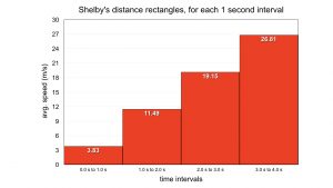
Notice that the distance rectangles of the speed versus time graph, taken together, appear like a triangle, sloping upward to the right, corresponding to speed increasing with time.
Half second time intervals
If we take a more precise look at the speeds, with half second intervals, the graph of speed versus time looks to be about the same size triangle, though more finely sliced. There are more rectangles, but they are skinnier: Δt, the base of the rectangle, is smaller.
Here is a table of average speeds in which to calculate distances, also.
| Time t (s) | Instantaneous speed (m/s) | Avg. speed (m/s) for this 0.5 second time interval |
avg. v Δt, Δt = 0.5 second | Displacement at time t (m) |
| 0 | 0.00 | 0 | ||
| ↓ | 1.915 | 0.9575 | ||
| 0.5 | 3.83 | 0.9575 | ||
| ↓ | 5.745 | 2.8725 | ||
| 1 | 7.66 | 3.83 | ||
| ↓ | 9.575 | 4.7875 | ||
| 1.5 | 11.49 | 8.6175 | ||
| ↓ | 13.405 | 6.7025 | ||
| 2 | 15.32 | 15.32 | ||
| ↓ | 17.235 | 8.6175 | ||
| 2.5 | 19.15 | 23.9375 | ||
| ↓ | 21.065 | 10.5325 | ||
| 3 | 22.98 | 34.47 | ||
| ↓ | 24.895 | 12.4475 | ||
| 3.5 | 26.81 | 46.9175 | ||
| ↓ | 28.725 | 14.3625 | ||
| 4 | 30.64 | 61.28 |
With skinnier time slices, more precision, there are eight distance rectangles.
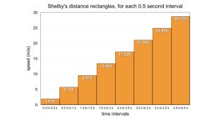
Remember: the rectangles are only approximations, though good, because they are based on average speeds.
Infinitesimal time intervals, instantaneous speed
Let’s see how the distance sum would change if we use instantaneous speeds. This will be an exact result, no approximation in the velocity diagram. The individual distance rectangles are now infinitesimally narrow, very small, so small that the graph of speed versus. time is no longer a jagged array of rectangles. It is a smooth triangle, just as smooth as the accelerating Shelby. The sum of all the areas of the red and orange distance rectangles above yield an estimate of the total displacement of the Shelby in 4.0 seconds, but here the area of the yellow triangle expresses the distance travelled.
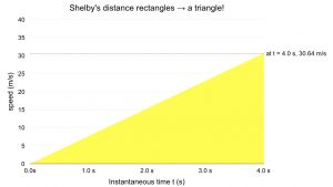
But now our area calculation is much simpler: one big triangle. In geometry class the area of a triangle whose base is  and whose height is
  takes a familiar form,
![\[A=\frac{1}{2}b\times h\]](https://pressbooks.online.ucf.edu/app/uploads/quicklatex/quicklatex.com-c1c8c291c7e35dcb24851a52ea320c24_l3.png "Rendered by QuickLaTeX.com")
Let’s break down this yellow triangle into motion concepts:
- In general its base is the elapsed time, . In the Shelby example,
 .
. - Its height is the amount of speed gained from rest,
 . In the Shelby example,

Therefore, using the familiar  triangle formula, but changed, mutatis mutandam, for the velocity graph’s triangle,
- the area of the yellow triangle is now interpreted as distance
 traveled;
 - its
 slope equates to the acceleration and
![\[d=\frac{1}{2}\Delta t \times a\Delta t\]](https://pressbooks.online.ucf.edu/app/uploads/quicklatex/quicklatex.com-0f6e4e196012e92dd3526c83b147f09e_l3.png "Rendered by QuickLaTeX.com")
![\[d=\frac{1}{2}a\left(\Delta t\right)^2\]](https://pressbooks.online.ucf.edu/app/uploads/quicklatex/quicklatex.com-5e5c2603e5b44f89de7a465e8a219201_l3.png "Rendered by QuickLaTeX.com")
I call this the distance triangle formula for an object starting up from rest,  . We will be using it frequently this semester. It is usually abbreviated as
  , without the , for brevity. In the example of the Shelby,
  .
.
Slowing down
If an object is slowing down as it moves across the x-axis, like a coin on a table sliding to a stop, the acceleration is a negative number. This negative signifies that the speed is decreasing over time. In the case of a slowdown acceleration, the slope of the velocity graph is negative, but the area still counts as a distance: the stopping distance. Here is the Shelby lightly touching the breaks,  , from initial speed
  . It takes about
  to slow down to a stop at this acceleration. The stopping distance is about
  .
.
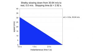
There are other formulas for distance calculations, especially important for handling the – negative sign in stopping accelerations and so forth, but  one will hold us for now.
1.15 How Do We Apply This Acceleration Concept? Where Do These Calculations Help Us Make Predictions?
We want to make descriptions and even predictions for the position of a baseball heading for the right field bleachers, the velocity of an proton in the Large Hadron Collider at CERN, the European Organization for Nuclear Research in Geneva, Switzerland. The nature of the prediction depends on the interaction: a baseball interacting with the gravitational field of Earth, a proton interacting with the magnetic field in an atom-smashing collider. So we need to follow Sir Isaac Newton’s instruction, “…from the phaenomena of motions to investigate the forces of nature…” And like Newton, himself, we must now look to Professor Galileo one more time, and gather up Galileo’s breakthrough ideas concerning states of motion. That will be our topic in the next chapter.