Main Body
Chapter 7, Oscillation: There and back again
©Thomas J. Brueckner 2017
What is an oscillation?
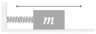
Something that moves back and forth in a periodic manner is an oscillating system. The simplest and easiest to understand is a coil spring attached at one end to something with a mass that can move and attached at the other end to a fixed point.
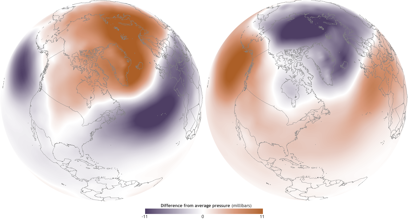
The image at the chapter’s beginning shows another kind of oscillating system, the Arctic Oscillation — in meteorological lingo, the AO. It is a pattern in atmospheric pressure, in which the atmospheric pressure over the Arctic shifts from above average pressure to below average pressure. During high pressure, the polar vortex is tight, and cold air stays up north. But as authors Caitlyn Kennedy and Rebecca Lindsey state,”At the other extreme, the conditions are reversed.” During lower pressure or “negative phase,” the polar vortex expands southward to the lower 48 states, and even Florida gets blasted with frigid weather. Kennedy and Lindsey mention that, previous to 2014, there was a large negative oscillation in the period December 2009-January 2010. I remember this from a day in the first week of January, when I dropped off my family at Orlando International Airport and absolutely froze!
Another atmospheric oscillation is something we hear every day: sound waves. Acoustic waves are very small variations in atmospheric pressure and density of the air between you, the observer, and the source. On a day when the barometric pressure is 1017.95 millibars, 30.06 inches of mercury, a sound wave propagates as a set of overpressures and underpressures, propagating from the source to your ear, as a set of densifications
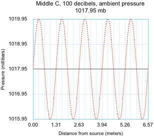
and rarefactions, to which your ear and brain respond by recognizing a pitch, in the frequency of the wave, 261.6 Hz, and by experiencing loudness, in the amplitude of the wave, 2 mb.
This pressure graph above displays a snapshot of the oscillating pressure value, above the ambient pressure 1017.95 mb, then below 1017.95 mb, then above, then below and so on for five cycles, fairly close to the source.
Note that this is a very small pressure oscillation, ±2 mb out of 1017.95 mb, or 0.2%. To see how small this is, we can zoom out from the small pressure window above to the full pressure scale, from zero millibars up to 1200 mb. The smooth wave shape above then becomes so flat that its plot looks like a flat line. Yet we humans can easily hear something at this intensity!
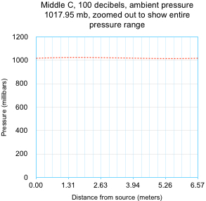
And another fact to keep in mind for both representations of the pressure wave: the speed of sound is about  . Each peak and each trough in the wave move across this 6.57 meter window in about 0.02 second!
Through the application of  and other laws of motion for O2 oxygen molecules and N2 nitrogen molecules in the air, coupled with lots of trigonometry and statistical formulae, a compact equation emerges, called the wave equation.
![\[v=\lambda f\]](https://pressbooks.online.ucf.edu/app/uploads/quicklatex/quicklatex.com-d2c3dc30c3b375617a6513549778f08e_l3.png "Rendered by QuickLaTeX.com")
It relates the wavelength  and frequency
  to the velocity of propagation,
 . Oscillating systems that generate waves frequently have a wave equation like this one.
Light is another oscillating system, electromagnetic radiation, but it is somewhat unusual in that it is a self-contained oscillating field. It is not a variation in a surrounding medium like sound waves in the medium of air. An oscillating electric charge, like an electron, generates an electric field and a magnetic field that couple together and propagate across a vacuum at the speed of light,  , which, for conversational purposes, we usually round off to
  . The wave equation for electromagnetic waves is
![\[c=\lambda f\]](https://pressbooks.online.ucf.edu/app/uploads/quicklatex/quicklatex.com-d1cfe47784cfcd22cc0a5068121b4e8a_l3.png "Rendered by QuickLaTeX.com")
,
which looks just like the generic wave equation above it. There is a significant caveat: this wave equation does not drop from F = ma and other principles as the wave equation for sound waves did. For light, there is no medium, there is only the electromagnetic field. We will talk more about light in the chapter on the electrodynamics.

“4.5′ Lift” by pzelez is licensed under CC BY-NC 2.0
So, having looked into many scientific topics so far, like electromagnetic and sound waves, we are now in position to study oscillation in the abstract. In terms of Newton’s three laws of motion, we can ask, “What kind of force produces oscillation?” Or, thinking four dimensionally, we can ask about the momentum and energy states of an oscillating system, “Does the potential energy of a spring have a position-related formula?” Our next two sections cover these questions.
What kind of force produces oscillation?
A force that keeps a spring-mass system oscillating back and forth, left to right then right to left — it has to be different than the Coulomb interaction. The Coulomb interaction stays attractive if oppositely-charged particles interact. They accelerate toward each other. Oppositely charged particles, like an electron and a

proton in a hydrogen atom, can take mutually oscillating paths with respect to each other, closer and farther and closer and farther. But the force never changes its direction — always toward the other particle.
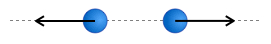
The Coulomb interaction also stays repulsive if two like-charged particles interact. They accelerate move away from each other. An electron moving toward another electron slows down because of repulsion, then stops, then turns around and moves off. But the force never changes direction — always away from the other particle.
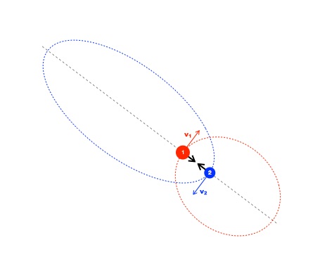
The gravitational interaction is always attractive, no matter the state of motion of two masses: if the two masses are initially moving apart, they only slow down and might turn around, a turning point in the motion. In astronomy, we see this all the time when looking at a binary star system, two enormous stars orbiting their center of mass on sometimes highly elliptical orbits, like Star 1 (red) and Star 2 (blue) in the diagram. But gravitational force never changes direction — always toward the other object.
Springs, however, are different.
For a spring-mass system, the force has to change direction, twice per cycle. When the system is at the
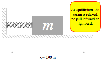
“relaxed” position, we call it equilibrium, where the spring ends up after friction drains off all kinetic energy. It is convenient to denote this position as the zero point of the oscillation axis: x = 0.00 m. At this position, the spring is just sitting there, slacking off, neither pushing or pulling.
However, when the mass is to the left of equilibrium, e.g., at x = -0.12 m, in red in the diagram below, the spring is compressed by 12 centimeters, 0.12 m, so the spring pushes back. For reference, the x = 0.00 m
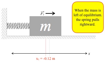
line is included in grey. The spring pushes the mass rightward with force F1. So the mass will accelerate rightward, and its Δv is rightward:
- if the mass is moving to the left, it slows down, but
- if the mass is moving to the right, it speeds up.
Going away from equilibrium to the left, it surrenders speed, but on the way back toward equilibrium, it recaptures speed. What happens when the mass is right of equilibrium?Say that you observe the mass moving on the right side of equilibrium and take a snapshot, at the exact moment its center of mass is 12 cm from
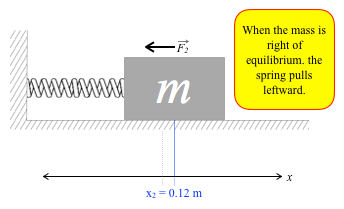
equilibrium, x = 0.12 m, in blue in the diagram below. Now the spring has been stretched out, and it wants to get back to slacking off status at equilibrium. Therefore the spring pulls left with force F2. Its acceleration will be leftward, and now the Δv is leftward:
- if the mass is moving to the left, it speeds up, but
- if the mass is moving to the right, it surrenders speed.
Now we can see how, as Kennedy and Lindsey wrote about the Arctic Oscillation, the spring-mass system also obeys the concept that “[at] the other extreme, the conditions are reversed.” On the right side of equilibrium, “the other extreme,” it surrenders kinetic energy when moving to the right but recaptures kinetic energy after it turns around and moves back to the left.
You might be saying to yourself, “Dr. Brueckner, did you say kinetic energy? Work?” Yes, I wrote it, and the energy states are always changing. But work is related to the force that does the work along some path with displacement Δx, so let’s look at the force law for springs.
The force law has to have a negative sign to encode the direction.
- When position is positive, the force is leftward, so it gets a negative sign.
- When position is negative, the force is rightward, and a negative sign changes a negative to positive for rightward direction.
The force law must also state the position dependence. In the 1600s, Robert Hooke figured out that for springs, the force is directly proportional to the displacement from equilibrium. This means that the force law is fairly simple:
![\[F=-kx\]](https://pressbooks.online.ucf.edu/app/uploads/quicklatex/quicklatex.com-2f766c35c000cb99f99289719cea7707_l3.png "Rendered by QuickLaTeX.com")
with a constant of proportionality  , known as the spring constant for a given spring. This makes the force a negative number of Newtons when x is positive — when the mass is right of equilibrium. Vice versa, the force is a positive number of Newtons when x is negative and the position of the mass is to the right of equilibrium.
The spring constant k encodes the relative stiffness of the spring. A really stiff coil spring like those for the suspension of a car, has very large values of . To get a lot of pushback force to support the weight of the car, a small displacement generates a big pushback. But if k is small, the spring is relatively soft. The same small displacement that got a lot of Newtons from the car’s spring will get you just a few Newtons, if k is smaller.
Here is an example, using a nice round number for the spring constant:  for the spring mentioned above, along with positions x1 = -0.12 m and x2 = 0.12 m. A spring of this stiffness might be useful in a small machine like a watch.
F1 = -k x1 = -(120 N/m)(-0.12 m) = 14.4 N. It is positive, a rightward force.
F2 = -kx2 = -(120 N/m)(0.12 m) = -14.4 N, negative, a leftward force.
If we move the object to another point, even further out, to x3 = 0.22 m, then the pull back force would be even stronger, F3 = -26.4 N.
A car’s coil spring might have a spring constant in the neighborhood of 80,000 N/m, which is equivalent to about 450 pounds per inch of compression. That would be fine for holding up a smaller car driving on a bumpy road.
Does the potential energy of a spring have a position-related formula?
A spring-mass system does obey a potential energy relation, and like all potential energy formulas, it depends on the position.
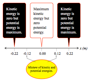
If you pull the mass out to x3 = 0.22 m, for instance and hold it there for a moment, its kinetic energy is zero. That is, you are holding it — it is at rest. When you release it, however, it builds up speed and heads leftward, back toward the equilibrium point. Its greatest acceleration leftward is at the moment you release it, because the pullback force is strongest there. Big Δv, so big change in kinetic energy.
As the mass goes left, the acceleration gets weaker. At x2, the pull back force was only 14.4 N, leftward. Therefore, in a given span of time, like 2 milliseconds, the Δv near x2 is smaller than out by x3. So the kinetic energy is still increasing, but not as quickly.
As the mass gets back to equilibrium, x = 0, the force goes to zero. At that instant of time, it stops accelerating leftward. This means it has reached maximum leftward velocity, and kinetic energy is maximum. But once it passes equilibrium, to negative x values, the spring pushes back, to the right, and though the mass is moving left, it slows down.
The mass keeps slowing down and by the time it reaches x4 = -0.22 m, it stops. It has given back all of its kinetic energy and the spring potential energy is maximum. The following diagram displays the basic energy concepts.
The spring potential energy and the kinetic energy vary by position, but not in the same way that gravitational potential energy does near the surface of Earth: -mgy. It requires a bit of fancy footwork with calculus to get the spring potential energy (SPE) formula:
![\[SPE=\frac{1}{2}kx^2\]](https://pressbooks.online.ucf.edu/app/uploads/quicklatex/quicklatex.com-c7591eb5082988d7c0369e3b58047fc8_l3.png "Rendered by QuickLaTeX.com")
With this formula we can now fill out a table of energy levels for the spring-mass system, including the total mechanical energy, E. And, let’s throw in one more position, x4 = -0.22 m, at the left hand turning point of the motion, and we will denote the center of the motion as xeq = 0.00 m, the equilibrium point.
|
Position |
x (meters) |
KE (Joules) |
SPE (Joules) |
E (Joules) |
|
x3 |
0.22 |
0.000 |
2.904 |
2.904 |
|
x2 |
0.12 |
2.040 |
0.864 |
2.904 |
|
xeq |
0.00 |
2.904 |
0.000 |
2.904 |
|
x1 |
-0.12 |
2.040 |
0.864 |
2.904 |
|
x4 |
-0.22 |
0.000 |
2.904 |
2.904 |
If we said that the mass is some number of kilograms, we could also calculate the speed at intermediate points x1 and x2, just as we did in the basketball free-fall calculations. E.g., what if the mass of the block is 0.008 kg, a little heavier than a nickel? Then what would the speed be at position x2?
Oscillators are everywhere!
Now that we have looked at the force law and the potential energy relation for the spring-mass system, we can wrap up this mini-chapter with a few comments.
The spring force is always pointing from the mass back toward the equilibrium point. For this reason we call it a restoring force.
Due to a nifty calculus result, we can say that any vibrating or oscillating system, no matter how complicated, can be approximated or simulated by a simple spring system,  and
and  , if the vibrations are fairly small. For this reason, engineers frequently study small vibrations diligently. Mechanical engineering students at UCF, for example, take a vibrations course, EML 4225 Introduction to Vibrations and Controls in their third year.
The generic term for the kind of oscillating system we’ve studied is simple harmonic oscillator, SHO.
Electronic circuits with a coil (inductance) and a pair of parallel metal plates (capacitor) form a simple harmonic oscillator — the voltage and current in the circuit oscillate. What a mass on a spring does on a table top, a circuit of this kind does when you hook it up to a volt meter or current meter. For this reason, some very elaborate electronic systems, and even computers, can be simulated by springs and masses and other mechanical objects.
Every physicist and engineer thinks an inordinate amount about oscillators, because oscillators are everywhere.